
7.4 用 Python 集成方法解决二分类问题
此节包含两个基本分类问题:二分类问题和多类别分类问题。二分类问题只有两种输出可能。输出可以是“点击广告”或者“不点击广告”。这里以岩石 vs. 水雷问题为例,利用声纳返回信号判断声纳扫描的是岩石还是水雷。
多类别分类问题是指有超过 2 个可能的输出。用根据玻璃化学成分对玻璃样本进行分类的问题来说明 Python 集成方法是如何解决此类问题的。
7.4.1 用 Python 随机森林方法探测未爆炸的水雷
下面列出了 RandomForestClassifier 类的构造函数及其参数。RandomForestClassifier的参数绝大多数与 RandomForestRegressor 的 一 样。RandomForestRegressor 的参数在用 RandomForestRegressor 对红酒口感进行预测的章节中已进行了讨论。这里只强调RandomForestClassifier 中的不同元素。
第一个不同是用于判断分割点质量的标准。回顾第 6 章中决策树的训练过程,需要尝试所有可能的属性,针对每个属性尝试所有可能的分割点,然后从中找出最佳的属性及其分割点。对于回归决策树,分割点的质量是由平方误差和( sum squared error)决定的。
但是平方误差和对于分类问题就不起作用了,需要类似误分类率的指标来描述。
下面是 sklearn.ensemble.RandomForestClassifier 类的构造函数。
sklearn.ensemble.RandomForestClassifier(n_estimators=10, criterion= 'gini', max_depth=None, min_samples_split=2, min_samples_leaf=1, max_features='auto', max_leaf_nodes=None, bootstrap=True, oob_score= False, n_jobs=1, random_state=None, verbose=0, min_density=None, compute_importances=None)
下面是对参数的描述。
✦ Criterion
字符串,可选(缺省值为“gini”)。
可能的取值如下。
Gini :利用基尼不纯度(Gini impurity)。
Entropy :利用基于熵的信息增益。
若想获得这两种评价方法的更多信息,可以访问 wikipedia 关于二元决策树的网页(http://en.wikipedia.org/wiki/Decision_tree_learning)。针对目前这个具体实例,这两者对集成方法性能的评价并没有太大的差异。
当训练数据终结于决策树的叶子节点时,叶子节点含有属于不同类别的数据,则根据叶子节点中不同类别的数据所占的百分比,分类决策树自然就可以得到数据属于某个类别的概率。依赖于具体的应用,可能想直接获得上述的概率,或者想直接将叶子节点中所占数据最多的类别作为预测值返回。如果在获得预测结果的同时想要调整阈值,则需要获得概率值。为了生成曲线下面积(area under the curve,AUC),可能想获得接收者操作特征曲线(receiver operating curve,ROC) 及其概率以保证精确度。如果想计算误分类率,则需要将概率转换为类别的预测。
下面是对方法的描述。
✦ Fit( X, y, sample_weight=None)
随机森林分类版本惟一的不同在于标签 y 的特征。对于分类问题,标签的取值为 0 到类别数减 1 的整数。对于二分类问题,标签的取值是 0 或 1。对于有 nClass 个不同类别的多类别分类问题,标签是从 0 到 nClass-1 的整数。
✦ Predict(X)
对于属性矩阵(二维的 numpy 数组)X,此函数产生所属类别的预测。它生成一个单列的数组,行数等于 X 的行数。每个元素是预测的所属类别,不管问题是二分类问题还是多类别分类问题,都是一样的。
✦ Predict_proba(X)
这个版本的预测函数产生一个二维数组。行数等于 X 的行数。列数就是预测的类别数(对于二分类问题就是 2 列)。每行的元素就是对应类别的概率。
✦ Predict_log_proba(X)
这个版本的预测函数产生一个与 predict_proba 相似的二维数组。但是显示的不是所属类别的概率,而是概率的 log 值。
7.4.2 构建随机森林模型探测未爆炸水雷
代码清单 7-8 展示了如何使用声纳数据构建随机森林模型来预测未爆炸的水雷。
数据的预处理和训练的过程与第 6 章和本章前面的随机森林的例子都很相似。不同之处主要在于这是一个分类问题。首先代码将标签从 M 和 R 转换成了 0 和 1。这是RandomForestClassifer 对输入数据的要求。其次训练完成后,在测试数据集上评价性能阶段。对于二分类问题,评价标准可以选择 ROC 曲线下面积(AUC),或者误分类率。如果可能的话,笔者通常倾向于使用 AUC,因为它能给出整体的性能评价。
为了计算 AUC,使用 predict_proba() 函数。如果预测输出为所属的类别,则不可能获得一个有用的 ROC 曲线(更准确地说,计算出的 ROC 曲线只有 3 个点,两端各 1 个点,中间 1 个点)。sklearn metric 工具包使得 AUC 的计算十分简单,只需要几行代码。代码将结果累积存入一个列表,然后绘出 AUC 性能与决策树数目的关系曲线图。代码清单 7-6绘制了 AUC 与决策树数目的关系图、30 个最重要属性的相对重要性排序、最大集成规模方法的 ROC 曲线图。代码的最后部分选取 3 个不同的阈值,打印输出针对每个阈值的混淆矩阵(Confusion Matrix)。阈值为 3 个四分位数,结果显示了当阈值从一个分位数转移到另外一个分位数时,假阳性、假阴性是如何变化的。
代码清单 7-6 随机森林分类岩石与水雷 -rocksVMinesRF.py
__author__ = 'mike_bowles'
import urllib2
from math import sqrt, fabs, exp
import matplotlib.pyplot as plot
from sklearn.cross_validation import train_test_split
from sklearn import ensemble
from sklearn.metrics import roc_auc_score, roc_curve
import numpy
#read data from uci data repository
target_url = ("https://archive.ics.uci.edu/ml/machine-learningdatabases/undocumented/connectionist-bench/sonar/sonar.all-data")
data = urllib2.urlopen(target_url)
#arrange data into list for labels and list of lists for attributes
xList = []
for line in data:
#split on comma
row = line.strip().split(",")
xList.append(row)
#separate labels from attributes, convert from attributes from
#string to numeric and convert "M" to 1 and "R" to 0
xNum = []
labels = []
for row in xList:
lastCol = row.pop()
if lastCol == "M":
labels.append(1)
else:
labels.append(0)
attrRow = [float(elt) for elt in row]
xNum.append(attrRow)
#number of rows and columns in x matrix
nrows = len(xNum)
ncols = len(xNum[1])
#form x and y into numpy arrays and make up column names
X = numpy.array(xNum)
y = numpy.array(labels)
rocksVMinesNames = numpy.array(['V' + str(i) for i in range(ncols)])
#break into training and test sets.
xTrain, xTest, yTrain, yTest = train_test_split(X, y, test_size=0.30,
random_state=531)
auc = []
nTreeList = range(50, 2000, 50)
for iTrees in nTreeList:
depth = None
maxFeat = 8 #try tweaking
rocksVMinesRFModel = ensemble.RandomForestClassifier(n_estimators=
iTrees, max_depth=depth, max_features=
maxFeat, oob_score=False, random_state=531)
rocksVMinesRFModel.fit(xTrain,yTrain)
#Accumulate auc on test set
prediction = rocksVMinesRFModel.predict_proba(xTest)
aucCalc = roc_auc_score(yTest, prediction[:,1:2])
auc.append(aucCalc)
print("AUC" )
print(auc[-1])
#plot training and test errors vs number of trees in ensemble
plot.plot(nTreeList, auc)
plot.xlabel('Number of Trees in Ensemble')
plot.ylabel('Area Under ROC Curve - AUC')
#plot.ylim([0.0, 1.1*max(mseOob)])
plot.show()
# Plot feature importance
featureImportance = rocksVMinesRFModel.feature_importances_
# normalize by max importance
featureImportance = featureImportance / featureImportance.max()
#plot importance of top 30
idxSorted = numpy.argsort(featureImportance)[30:60]
idxTemp = numpy.argsort(featureImportance)[::-1]
print(idxTemp)
barPos = numpy.arange(idxSorted.shape[0]) + .5
plot.barh(barPos, featureImportance[idxSorted], align='center')
plot.yticks(barPos, rocksVMinesNames[idxSorted])
plot.xlabel('Variable Importance')
plot.show()
#plot best version of ROC curve
fpr, tpr, thresh = roc_curve(yTest, list(prediction[:,1:2]))
ctClass = [i*0.01 for i in range(101)]
plot.plot(fpr, tpr, linewidth=2)
plot.plot(ctClass, ctClass, linestyle=':')
plot.xlabel('False Positive Rate')
plot.ylabel('True Positive Rate')
plot.show()
#pick some threshold values and calc confusion matrix for
#best predictions
#notice that GBM predictions don't fall in range of (0, 1)
#pick threshold values at 25th, 50th and 75th percentiles
idx25 = int(len(thresh) * 0.25)
idx50 = int(len(thresh) * 0.50)
idx75 = int(len(thresh) * 0.75)
#calculate total points, total positives and total negatives
totalPts = len(yTest)
P = sum(yTest)
N = totalPts - P
print('')
print('Confusion Matrices for Different Threshold Values')
#25th
TP = tpr[idx25] * P; FN = P - TP; FP = fpr[idx25] * N; TN = N - FP
print('')
print('Threshold Value = ', thresh[idx25])
print('TP = ', TP/totalPts, 'FP = ', FP/totalPts)
print('FN = ', FN/totalPts, 'TN = ', TN/totalPts)
#50th
TP = tpr[idx50] * P; FN = P - TP; FP = fpr[idx50] * N; TN = N - FP
print('')
print('Threshold Value = ', thresh[idx50])
print('TP = ', TP/totalPts, 'FP = ', FP/totalPts)
print('FN = ', FN/totalPts, 'TN = ', TN/totalPts)
#75th
TP = tpr[idx75] * P; FN = P - TP; FP = fpr[idx75] * N; TN = N - FP
print('')
print('Threshold Value = ', thresh[idx75])
print('TP = ', TP/totalPts, 'FP = ', FP/totalPts)
print('FN = ', FN/totalPts, 'TN = ', TN/totalPts)
# Printed Output:
#
# AUC
# 0.950304259635
#
# Confusion Matrices for Different Threshold Values
#
# ('Threshold Value = ', 0.76051282051282054)
# ('TP = ', 0.25396825396825395, 'FP = ', 0.0)
# ('FN = ', 0.2857142857142857, 'TN = ', 0.46031746031746029)
#
# ('Threshold Value = ', 0.62461538461538457)
# ('TP = ', 0.46031746031746029, 'FP = ', 0.047619047619047616)
# ('FN = ', 0.079365079365079361, 'TN = ', 0.41269841269841268)
#
# ('Threshold Value = ', 0.46564102564102566)
# ('TP = ', 0.53968253968253965, 'FP = ', 0.22222222222222221)
# ('FN = ', 0.0, 'TN = ', 0.23809523809523808)
7.4.3 随机森林分类器的性能
图 7-13 为 AUC 与决策树数目的关系图。此图是以往看过的均方误差或误分类错误与决策树数目关系图的倒置。对于均方误差和误分类错误,值越小越好。对于 AUC 来说,1.0是相当完美的,但是 0.5 就很差了。因此,AUC 值越大越好,不是寻找曲线中的波谷,而是找波峰。图 7-13 展示在曲线的左侧出现了一个波峰。然而,因为随机森林只减少方差,不会过拟合,因此波峰也可以归功于随机的波动。正像本章早期的回归问题,最佳模型是包含所有决策树的模型,其性能是图中最右的点。
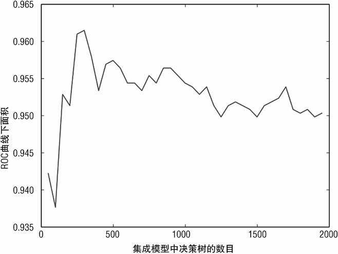
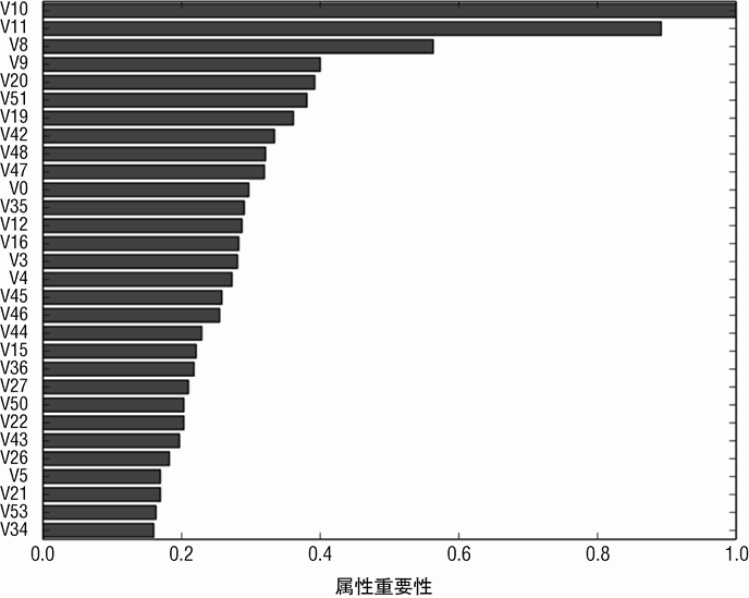
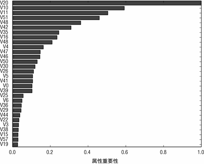
图 7-14 是最重要的前 30 个属性的重要性排名。在水雷检测的问题中,不同的属性对应不同频率的声纳信号,即不同波长的信号。如果要求设计一个机器学习系统来解决这个问题,下一步就是确定这些属性对应的波长,确定波长与水雷和岩石在不同维度上的对应关系。这样可以加深对模型的理解。
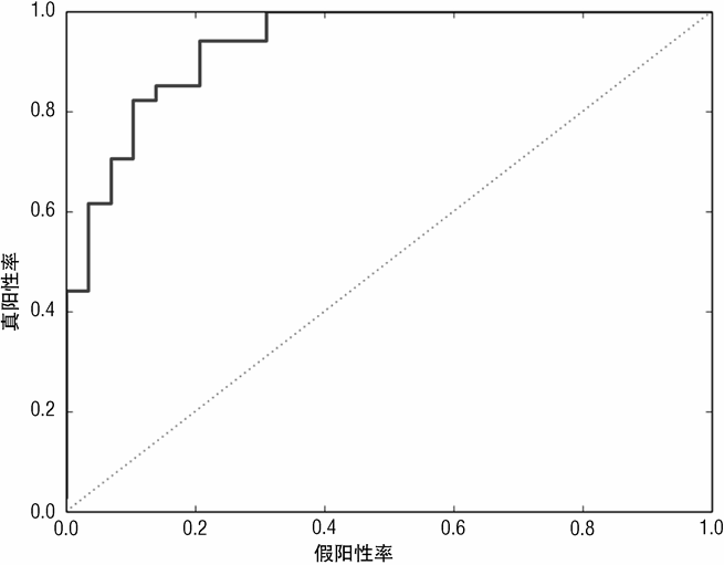
此模型的 AUC 值相当高,其 ROC 曲线表现也相当好。虽然还达不到左上角,但也十分接近。
7.4.4 用 Python 梯度提升法探测未爆炸水雷
代码清单 7-7 为 scikitlearn 中梯度提升法的构造函数。绝大多数 GradientBoosting Classifer 的参数和方法与 GradientBoostingRegressor 的相同。下面主要描述其不同的参数和方法。
下面是 sklearn.ensemble.GradientBoostingClassifier 类的构造函数。
sklearn.ensemble.GradientBoostingClassifier(loss='deviance', learning_rate=0.1, n_estimators=100, subsample=1.0, min_samples_split=2,min_samples_leaf=1, max_depth=3, init=None, random_state=None, max_features=None, verbose=0, max_leaf_nodes=None, warm_start=False)
下面是对参数的描述。
✦ loss
deviance 对于分类问题,deviance 是缺省的,也是唯一的选项。
下面是对方法的描述。
✦ fit(X,y , monitor=None)
对于分类问题,其不同点只在于标签 y 的不同。对应分类问题,标签是 0 到类别总数减 1 的一个整数。对于二分类问题,标签值为0或者 1。对于多类别分类问题,如果共有nClass 个不同的类别,则标签取值为 0 ~ nClass-1。
✦ decision_function(X)
梯度提升分类器实际上是回归决策树的集合,会产生与所属类别的概率相关的实数估计值。这些估计值还需要经过反 logistic 函数将其转换为概率。转换前的实数估计值可通过此函数获得,对这些估计值的使用就像 ROC 曲线计算中使用概率那样简单。
✦ predict(X)
此函数预测所属类别。
✦ predict_proba(X)
此函数预测所属类别的概率。它对于每个类别有一列概率值。对于二分类问题有两列。
对于多类别分类问题,共有 nClass 列。
上述函数的阶段性(staged)版本是可迭代的,产生与决策树数目相同的结果(也与训练过程中执行的步数一致)。
✦ staged_decison_function(X)
此为 decision 函数的可迭代版本。
✦ staged_predict(X)
此为 predict 函数的可迭代版本。
✦ staged_predict_proba(X)
此为 predict_proba 函数的可迭代版本。
代码清单 7-7 使用 sklearn 的 GradientBoostingClassifier 完成探测未爆炸水雷的任务。
代码清单 7-7 梯度提升法分类岩石与水雷 -rocksVMinesGBM.py
__author__ = 'mike_bowles'
import urllib2
from math import sqrt, fabs, exp
import matplotlib.pyplot as plot
from sklearn.cross_validation import train_test_split
from sklearn import ensemble
from sklearn.metrics import roc_auc_score, roc_curve
import numpy
#read data from uci data repository
target_url = ("https://archive.ics.uci.edu/ml/machine-learning-databases/undocumented/connectionist-bench/sonar/sonar.all-data")
data = urllib2.urlopen(target_url)
#arrange data into list for labels and list of lists for attributes
xList = []
for line in data:
#split on comma
row = line.strip().split(",")
xList.append(row)
#separate labels from attributes, convert from attributes from
#string to numeric and convert "M" to 1 and "R" to 0
xNum = []
labels = []
for row in xList:
lastCol = row.pop()
if lastCol == "M":
labels.append(1)
else:
labels.append(0)
attrRow = [float(elt) for elt in row]
xNum.append(attrRow)
#number of rows and columns in x matrix
nrows = len(xNum)
ncols = len(xNum[1])
#form x and y into numpy arrays and make up column names
X = numpy.array(xNum)
y = numpy.array(labels)
rockVMinesNames = numpy.array(['V' + str(i) for i in range(ncols)])
#break into training and test sets.
xTrain, xTest, yTrain, yTest = train_test_split(X, y, test_size=0.30,
random_state=531)
#instantiate model
nEst = 2000
depth = 3
learnRate = 0.007
maxFeatures = 20
rockVMinesGBMModel = ensemble.GradientBoostingClassifier(
n_estimators=nEst, max_depth=depth,
learning_rate=learnRate,
max_features=maxFeatures)
#train
rockVMinesGBMModel.fit(xTrain, yTrain)
# compute auc on test set as function of ensemble size
auc = []
aucBest = 0.0
predictions = rockVMinesGBMModel.staged_decision_function(xTest)
for p in predictions:
aucCalc = roc_auc_score(yTest, p)
auc.append(aucCalc)
#capture best predictions
if aucCalc > aucBest:
aucBest = aucCalc
pBest = p
idxBest = auc.index(max(auc))
#print best values
print("Best AUC" )
print(auc[idxBest])
print("Number of Trees for Best AUC")
print(idxBest)
#plot training deviance and test auc's vs number of trees in ensemble
plot.figure()
plot.plot(range(1, nEst + 1), rockVMinesGBMModel.train_score_,
label='Training Set Deviance', linestyle=":")
plot.plot(range(1, nEst + 1), auc, label='Test Set AUC')
plot.legend(loc='upper right')
plot.xlabel('Number of Trees in Ensemble')
plot.ylabel('Deviance / AUC')
plot.show()
# Plot feature importance
featureImportance = rockVMinesGBMModel.feature_importances_
# normalize by max importance
featureImportance = featureImportance / featureImportance.max()
#plot importance of top 30
idxSorted = numpy.argsort(featureImportance)[30:60]
barPos = numpy.arange(idxSorted.shape[0]) + .5
plot.barh(barPos, featureImportance[idxSorted], align='center')
plot.yticks(barPos, rockVMinesNames[idxSorted])
plot.xlabel('Variable Importance')
plot.show()
#pick threshold values and calc confusion matrix for best predictions
#notice that GBM predictions don't fall in range of (0, 1)
#plot best version of ROC curve
fpr, tpr, thresh = roc_curve(yTest, list(pBest))
ctClass = [i*0.01 for i in range(101)]
plot.plot(fpr, tpr, linewidth=2)
plot.plot(ctClass, ctClass, linestyle=':')
plot.xlabel('False Positive Rate')
plot.ylabel('True Positive Rate')
plot.show()
#pick threshold values and calc confusion matrix for best predictions
#notice that GBM predictions don't fall in range of (0, 1)
#pick threshold values at 25th, 50th and 75th percentiles
idx25 = int(len(thresh) * 0.25)
idx50 = int(len(thresh) * 0.50)
idx75 = int(len(thresh) * 0.75)
#calculate total points, total positives and total negatives
totalPts = len(yTest)
P = sum(yTest)
N = totalPts - P
print('')
print('Confusion Matrices for Different Threshold Values')
#25th
TP = tpr[idx25] * P; FN = P - TP; FP = fpr[idx25] * N; TN = N - FP
print('')
print('Threshold Value = ', thresh[idx25])
print('TP = ', TP/totalPts, 'FP = ', FP/totalPts)
print('FN = ', FN/totalPts, 'TN = ', TN/totalPts)
#50th
TP = tpr[idx50] * P; FN = P - TP; FP = fpr[idx50] * N; TN = N - FP
print('')
print('Threshold Value = ', thresh[idx50])
print('TP = ', TP/totalPts, 'FP = ', FP/totalPts)
print('FN = ', FN/totalPts, 'TN = ', TN/totalPts)
#75th
TP = tpr[idx75] * P; FN = P - TP; FP = fpr[idx75] * N; TN = N - FP
print('')
print('Threshold Value = ', thresh[idx75])
print('TP = ', TP/totalPts, 'FP = ', FP/totalPts)
print('FN = ', FN/totalPts, 'TN = ', TN/totalPts)
# Printed Output:
#
# Best AUC
# 0.936105476673
# Number of Trees for Best AUC
# 1989
#
# Confusion Matrices for Different Threshold Values
#
# ('Threshold Value = ', 6.2941249291909935)
# ('TP = ', 0.23809523809523808, 'FP = ', 0.015873015873015872)
# ('FN = ', 0.30158730158730157, 'TN = ', 0.44444444444444442)
#
# ('Threshold Value = ', 2.2710265370949441)
# ('TP = ', 0.44444444444444442, 'FP = ', 0.063492063492063489)
# ('FN = ', 0.095238095238095233, 'TN = ', 0.3968253968253968)
#
# ('Threshold Value = ', -3.0947902666953317)
# ('TP = ', 0.53968253968253965, 'FP = ', 0.22222222222222221)
# ('FN = ', 0.0, 'TN = ', 0.23809523809523808)
#
#
# Printed Output with max_features = 20 (Random Forest base learners):
#
# Best AUC
# 0.956389452333
# Number of Trees for Best AUC
# 1426
#
# Confusion Matrices for Different Threshold Values
#
# ('Threshold Value = ', 5.8332200248698536)
# ('TP = ', 0.23809523809523808, 'FP = ', 0.015873015873015872)
# ('FN = ', 0.30158730158730157, 'TN = ', 0.44444444444444442)
#
# ('Threshold Value = ', 2.0281780133610567)
# ('TP = ', 0.47619047619047616, 'FP = ', 0.031746031746031744)
# ('FN = ', 0.063492063492063489, 'TN = ', 0.42857142857142855)
#
# ('Threshold Value = ', -1.2965629080181333)
# ('TP = ', 0.53968253968253965, 'FP = ', 0.22222222222222221)
# ('FN = ', 0.0, 'TN = ', 0.23809523809523808)
此代码的流程与随机森林的基本相同。一个不同点是梯度提升法会过拟合,因此当代码累积计算 AUC 并将其存入一个列表准备绘制时,程序同时持续跟踪 AUC 的最佳值。
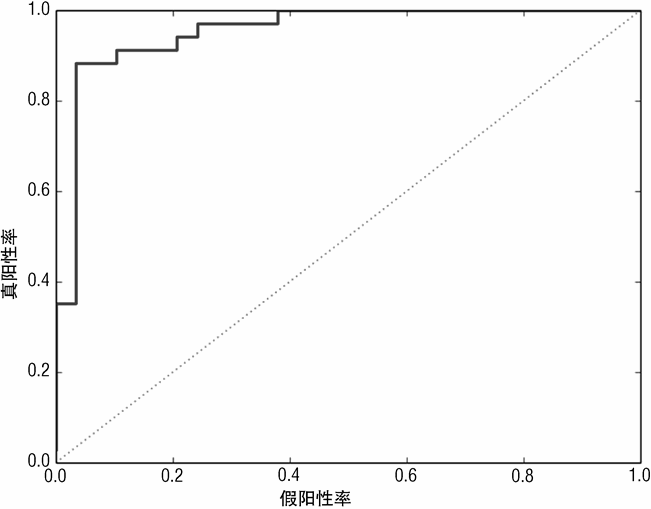
其最佳值用来生成 ROC 曲线、假阳性、假阴性等指标(如图 7-15 所示)。另一个不同是梯度提升方法运行了 2 次,一次是使用普通的决策树,另外一次是使用随机森林基学习器。
两者都获得了很好的分类性能。使用随机森林基学习器的性能更好,这点与鲍鱼预测年龄问题不同。在鲍鱼预测年龄问题上,采用随机森林基学习器并没有获得显著的改善。
7.4.5 梯度提升法分类器的性能
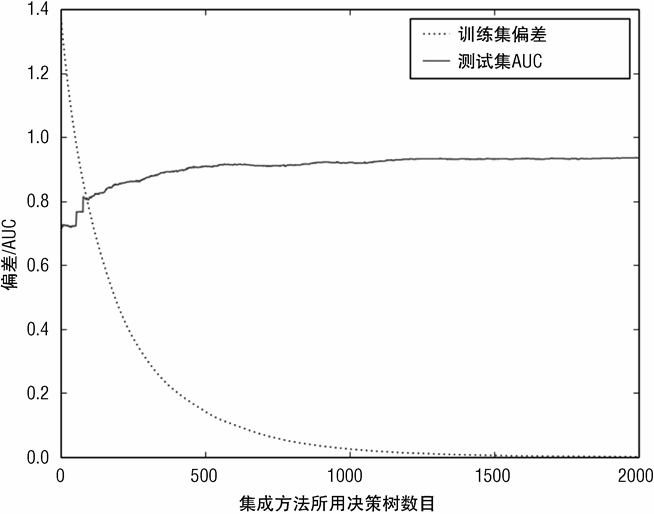
图 7-16 绘制了两个曲线。一个是训练集的偏差(deviance)。偏差与估计值距离正确值有多远相关,但又与误分类误差稍微有些差别。把偏差绘制出来是因为梯度提升法就是把偏差作为优化的目标。在图中可以看到训练过程中偏差的变化。AUC(基于测试数据)也在图中绘出是为了展示随着决策树数目的增加测试数据的性能的变化(决策树数目的增加就等同于在梯度下降中采取了更多的步骤;每一步就意味着又训练了一个决策树)。
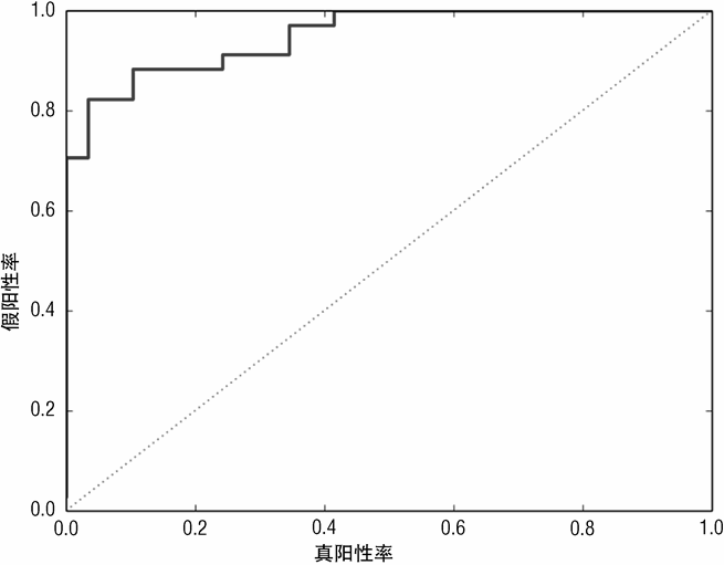
图 7-17 绘制了最重要的前 30 个属性的重要性排名。图 7-17 中的属性重要性排名与随机森林的(见图 7-14)有些不同,但是也有共同点,如属性 V10、V11、V20 和 V51 排名都比较靠前,尽管具体的顺序可能不同。
使用随机森林基学习器的梯度提升法的模型训练过程如图 7-18,7-19 所示。使用随机森林基学习器确实获得了更好的结果,但是这种差异还不足以在图中有所体现。

通过比较图 7-20 与图 7-17 可知使用随机森林基学习器对属性的重要性影响不大。
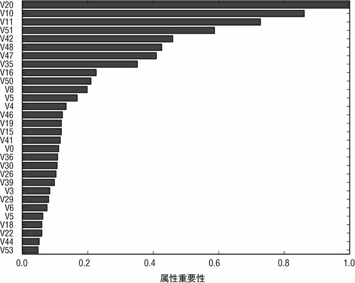
图 7-21 为使用随机森林基学习器的梯度提升法检测水雷的 ROC 曲线。
此节介绍了如何用集成方法解决二分类问题。在很多方面,使用集成方法解决二分类问题与回归问题基本相同,可以注意到初始化 RandomForestRegressor 所需的参数与初始化 RandomForestClassification 的基本一样。基于第 6 章的介绍,就可以理解这种一致背后的原因。
集成方法用于分类问题和回归问题的不同之处主要在于对误差的评价方法和误差特征的刻画不同。
下节主要介绍上述方法如何解决多类别分类问题。


本书评论