
7.3 Python 集成方法引入非数值属性
非数值属性是指那些取某几个离散非数值型的属性。人口普查记录就含有大量的非数值属性,“已婚、单身或离异”就是一个例子,家庭住址所在州则是另外一个例子。非数值属性可以提高预测的准确性,但是 Python 集成方法实现需要数值型输入数据。第 4 章和第5 章介绍了如何对因素变量编码,使其能够引入惩罚线性回归模型。在此也可以采用同样的技术。本节以预测鲍鱼年龄问题为例说明如何应用此项技术。
7.3.1 对鲍鱼性别属性编码引入Python 随机森林回归方法
假设有一个可以取 n 个值的属性。例如,属性“美国的州”就有 50 个取值,“婚姻状况”有 3 个取值。对于一个有 n 个取值的因素变量,可以创建 n−1 个新的虚拟属性。当变量取第 i 个值时,第 i 个虚拟属性置为 1,其他的虚拟属性置为 0。如果变量取第 n 个值,则所有虚拟变量都置为 0。鲍鱼数据将对此进行详细说明。
代码清单 7-4 展示了利用鲍鱼的重量、壳的尺寸等属性来训练随机森林模型,然后利用模型预测鲍鱼的年龄。此问题的目标是基于各种物理测量指标(鲍鱼各个部分的重量、鲍鱼的尺寸等)来预测鲍鱼的年龄。预测红酒口感的算法也可以用于这个回归问题。
代码清单 7-4 随机森林方法预测鲍鱼年龄 -abaloneRF.py
__author__ = 'mike_bowles'
import urllib2
from pylab import *
import matplotlib.pyplot as plot
import numpy
from sklearn.cross_validation import train_test_split
from sklearn import ensemble
from sklearn.metrics import mean_squared_error
target_url = ("http://archive.ics.uci.edu/ml/machine-learning-databases/abalone/abalone.data")
#read abalone data
data = urllib2.urlopen(target_url)
xList = []
labels = []
for line in data:
#split on semi-colon
row = line.strip().split(",")
#put labels in separate array and remove label from row
labels.append(float(row.pop()))
#form list of list of attributes (all strings)
xList.append(row)
#code three-valued sex attribute as numeric
xCoded = []
for row in xList:
#first code the three-valued sex variable
codedSex = [0.0, 0.0]
if row[0] == 'M': codedSex[0] = 1.0
if row[0] == 'F': codedSex[1] = 1.0
numRow = [float(row[i]) for i in range(1,len(row))]
rowCoded = list(codedSex) + numRow
xCoded.append(rowCoded)
#list of names for
abaloneNames = numpy.array(['Sex1', 'Sex2', 'Length', 'Diameter',
'Height', 'Whole weight', 'Shucked weight', 'Viscera weight',
'Shell weight', 'Rings'])
#number of rows and columns in x matrix
nrows = len(xCoded)
ncols = len(xCoded[1])
#form x and y into numpy arrays and make up column names
X = numpy.array(xCoded)
y = numpy.array(labels)
#break into training and test sets.
xTrain, xTest, yTrain, yTest = train_test_split(X, y, test_size=0.30,
random_state=531)
#train Random Forest at a range of ensemble sizes in
#order to see how the mse changes
mseOos = []
nTreeList = range(50, 500, 10)
for iTrees in nTreeList:
depth = None
maxFeat = 4 #try tweaking
abaloneRFModel = ensemble.RandomForestRegressor(n_estimators=iTrees,
max_depth=depth, max_features=maxFeat,
oob_score=False, random_state=531)
abaloneRFModel.fit(xTrain,yTrain)
#Accumulate mse on test set
prediction = abaloneRFModel.predict(xTest)
mseOos.append(mean_squared_error(yTest, prediction))
print("MSE" )
print(mseOos[-1])
#plot training and test errors vs number of trees in ensemble
plot.plot(nTreeList, mseOos)
plot.xlabel('Number of Trees in Ensemble')
plot.ylabel('Mean Squared Error')
#plot.ylim([0.0, 1.1*max(mseOob)])
plot.show()
# Plot feature importance
featureImportance = abaloneRFModel.feature_importances_
# normalize by max importance
featureImportance = featureImportance / featureImportance.max()
sortedIdx = numpy.argsort(featureImportance)
barPos = numpy.arange(sortedIdx.shape[0]) + .5
plot.barh(barPos, featureImportance[sortedIdx], align='center')
plot.yticks(barPos, abaloneNames[sortedIdx])
plot.xlabel('Variable Importance')
plot.subplots_adjust(left=0.2, right=0.9, top=0.9, bottom=0.1)
plot.show()
# Printed Output:
# MSE
# 4.30971555911
此数据集的一个属性就是鲍鱼的性别。鲍鱼的性别有三个可能的取值:雄性、雌性和未成年(一个鲍鱼的性别在幼年期间是不确定的)。因此性别属性是一个三值因素变量。
在数据集中,性别属性是 3 个字符变量:M、F 和 I。代码首先定义了一个列表,缺省设置为 2 个浮点型的 0。如果属性值是 M,则列表第一个元素的值变为 1.0。如果属性值是 F,则列表第二个元素的值变为 1.0。否则,此列表就是 2 个零值(即当属性值是 I 时)。然后用这个新的两个元素的列表来代替原来的字符变量,结果用于构建随机森林模型。
7.3.2 评估性能以及变量编码的重要性
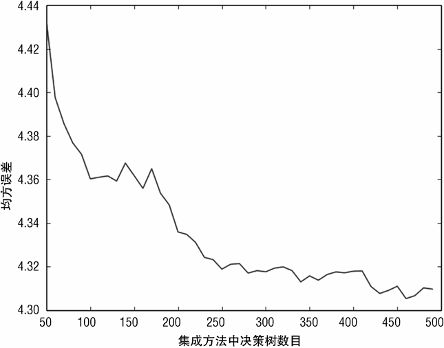
图 7-7 展示了随着随机森林集成方法中决策树数目的变化,均方误差是如何减少的。
均方误差最小值为 4.31。正如第 2 章关于鲍鱼数据的统计信息所述,鲍鱼年龄(鲍鱼壳上的年轮)的标准差(standard deviation)为 3.22,则其方差为 10.37。因此,针对此数据集,随机森林大约可以预测年龄方差变化的 58%。
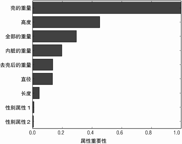
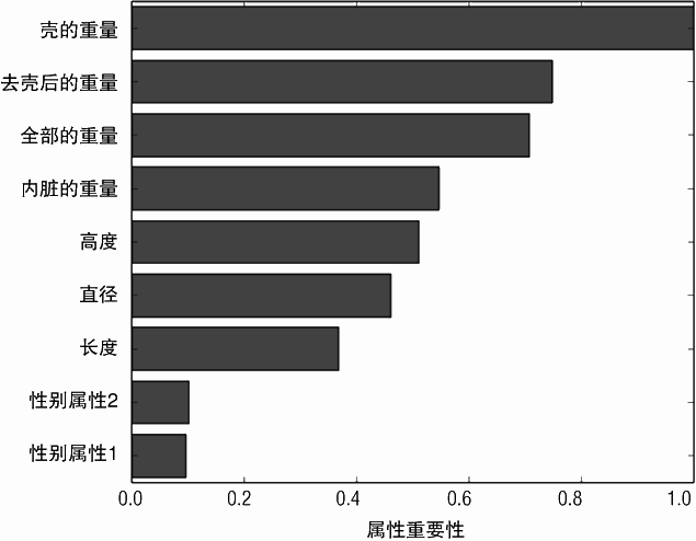
对于随机森林模型属性的相对重要性如图 7-8 所示。由性别创建的两个属性:性别属性 1 和性别属性 2 在这个模型中并不是非常重要的。
7.3.3 在梯度提升回归方法中引入鲍鱼性别属性
梯度提升法对性别变量的处理与随机森林一样。代码清单 7-5 包含了训练梯度提升模型的代码。
代码清单 7-5 用梯度提升法预测鲍鱼年龄 -abaloneGBM.py
__author__ = 'mike_bowles'
import urllib2
from pylab import *
import matplotlib.pyplot as plot
import numpy
from sklearn.cross_validation import train_test_split
from sklearn import ensemble
from sklearn.metrics import mean_squared_error
target_url = ("http://archive.ics.uci.edu/ml/machine-learning-databases/abalone/abalone.data")
#read abalone data
data = urllib2.urlopen(target_url)
xList = []
labels = []
for line in data:
#split on semi-colon
row = line.strip().split(",")
#put labels in separate array and remove label from row
labels.append(float(row.pop()))
#form list of list of attributes (all strings)
xList.append(row)
#code three-valued sex attribute as numeric
xCoded = []
for row in xList:
#first code the three-valued sex variable
codedSex = [0.0, 0.0]
if row[0] == 'M': codedSex[0] = 1.0
if row[0] == 'F': codedSex[1] = 1.0
numRow = [float(row[i]) for i in range(1,len(row))]
rowCoded = list(codedSex) + numRow
xCoded.append(rowCoded)
#list of names for
abaloneNames = numpy.array(['Sex1', 'Sex2', 'Length', 'Diameter',
'Height', 'Whole weight', 'Shucked weight',
'Viscera weight', 'Shell weight', 'Rings'])
#number of rows and columns in x matrix
nrows = len(xCoded)
ncols = len(xCoded[1])
#form x and y into numpy arrays and make up column names
X = numpy.array(xCoded)
y = numpy.array(labels)
#break into training and test sets.
xTrain, xTest, yTrain, yTest = train_test_split(X, y, test_size=0.30,
random_state=531)
#instantiate model
nEst = 2000
depth = 5
learnRate = 0.005
maxFeatures = 3
subsamp = 0.5
abaloneGBMModel = ensemble.GradientBoostingRegressor(n_estimators=nEst,
max_depth=depth, learning_rate=learnRate,
max_features=maxFeatures,subsample=subsamp,
loss='ls')
#train
abaloneGBMModel.fit(xTrain, yTrain)
# compute mse on test set
msError = []
predictions = abaloneGBMModel.staged_decision_function(xTest)
for p in predictions:
msError.append(mean_squared_error(yTest, p))
print("MSE" )
print(min(msError))
print(msError.index(min(msError)))
#plot training and test errors vs number of trees in ensemble
plot.figure()
plot.plot(range(1, nEst + 1), abaloneGBMModel.train_score_,
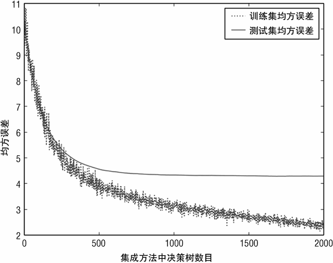
label='Training Set MSE', linestyle=":")
plot.plot(range(1, nEst + 1), msError, label='Test Set MSE')
plot.legend(loc='upper right')
plot.xlabel('Number of Trees in Ensemble')
plot.ylabel('Mean Squared Error')
plot.show()
# Plot feature importance
featureImportance = abaloneGBMModel.feature_importances_
# normalize by max importance
featureImportance = featureImportance / featureImportance.max()
idxSorted = numpy.argsort(featureImportance)
barPos = numpy.arange(idxSorted.shape[0]) + .5
plot.barh(barPos, featureImportance[idxSorted], align='center')
plot.yticks(barPos, abaloneNames[idxSorted])
plot.xlabel('Variable Importance')
plot.subplots_adjust(left=0.2, right=0.9, top=0.9, bottom=0.1)
plot.show()
# Printed Output:
# for Gradient Boosting
# nEst = 2000
# depth = 5
# learnRate = 0.003
# maxFeatures = None
# subsamp = 0.5
#
# MSE
# 4.22969363284
# 1736
#for Gradient Boosting with RF base learners
# nEst = 2000
# depth = 5
# learnRate = 0.005
# maxFeatures = 3
# subsamp = 0.5
#
# MSE
# 4.27564515749
# 1687
7.3.4 梯度提升法的性能评价以及变量编码的重要性
训练和预测中的注意事项如下。
(1)查看梯度提升法中各属性的重要性排名,看看编码后的性别属性是否重要。
(2)查看将随机森林基学习器引入梯度提升的 Python 实现。这会带来性能提升还是下降?让梯度提升法使用随机森林基学习器只需要改变 max_features 参数,将其从 None变成一个小于属性总数目的一个整数,或者是小于 1.0 的一个浮点数。当 max_featues 设为 None 时,在决策树生长的过程中,在每个节点寻找最佳的属性以分割数据时,全部 9个属性是都要考虑的。当 max_features 设为小于 9 的整数,在每个节点进行数据分割时,是随机选择 max_features 个属性来考虑的。
代码清单 7-5 的输出结果显示在代码清单的最后。通过均方误差可以看出随机森林和梯度提升对鲍鱼年龄预测问题来说性能上没有显著的差异。梯度提升法使用简单的决策树还是使用随机森林作为基学习器对性能来说也没有显著的差异。
采用简单的决策树还是随机森林作为基学习器,从预测误差和集成方法规模的关系曲线上来看也几乎没有差别,这个从图 7-9 ~图 7-11 之间的对比就可以看出。
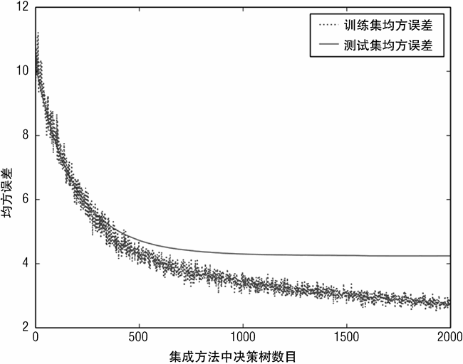
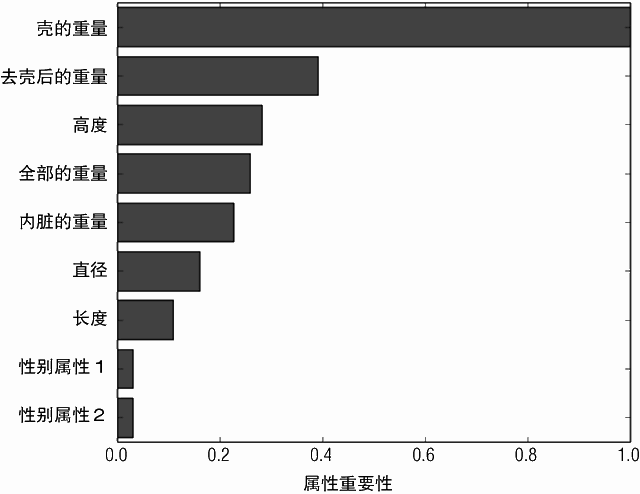
图 7-10 和图 7-12 分别展示了基于简单决策树和随机森林的梯度提升法属性的相对重要性的排名。两者之间唯一的差别就是属性“内脏的重量”和“高度”( 第 4 和第 5 个最重要属性)互换了位置。相似地,随机森林中属性的重要性排名和这两个梯度提升法的也几乎没有差别。
有看法认为,随机森林适合于规模很大且很稀疏的属性空间,如文本挖掘问题。下节主要比较这两种算法在分类问题上的表现:利用声纳输出将岩石和水雷区分开来。这个问题有 60 个属性,虽然不如文本挖掘问题的属性种类多,但是可能会展示出这两种梯度提升法(基于二元决策树的梯度提升法和基于随机森林基学习器的梯度提升法)在性能上的差异。


本书评论