7.5 用 Python 集成方法解决多类别分类问题
Python 实现的随机森林和梯度提升可以构建二分类和多类别分类模型。这两个模型之间有天然的差别。首先是标签(y)。随机森林和梯度提升的讨论就包含对标签的处理。
对于一个有 nClass 个不同类别的分类问题,标签取0~ nClass-1 的整数。另外一个体现类别数量的是不同预测方法的输出。预测所属类别的方法输出与标签相同范围的整数值,预测所属类别概率的方法输出为 nClass 个可能类别对应的概率。
另外一个需要关注差异性的领域就是对性能的评价。误分类错误仍然是有意义的,在此节将看到基于误分类错误评价测试数据性能的代码。当类别超过两个时,AUC 的使用将更复杂,不同误差类型之间的权衡也将更有挑战性。
7.5.1 用随机森林对玻璃进行分类
代码清单 7-8 遵循的流程与用于探测水雷的代码基本一致。
代码清单 7-8 用随机森林对玻璃进行分类 -glassRF.py
__author__ = 'mike_bowles'
import urllib2
from math import sqrt, fabs, exp
import matplotlib.pyplot as plot
from sklearn.linear_model import enet_path
from sklearn.metrics import accuracy_score, confusion_matrix, roc_curve
from sklearn.cross_validation import train_test_split
from sklearn import ensemble
import numpy
target_url = ("https://archive.ics.uci.edu/ml/machine-learning-databases/glass/glass.data")
data = urllib2.urlopen(target_url)
#arrange data into list for labels and list of lists for attributes
xList = []
for line in data:
#split on comma
row = line.strip().split(",")
xList.append(row)
glassNames = numpy.array(['RI', 'Na', 'Mg', 'Al', 'Si', 'K', 'Ca',
'Ba', 'Fe', 'Type'])
#Separate attributes and labels
xNum = []
labels = []
for row in xList:
labels.append(row.pop())
l = len(row)
#eliminate ID
attrRow = [float(row[i]) for i in range(1, l)]
xNum.append(attrRow)
#number of rows and columns in x matrix
nrows = len(xNum)
ncols = len(xNum[1])
#Labels are integers from 1 to 7 with no examples of 4.
#gb requires consecutive integers starting at 0
newLabels = []
labelSet = set(labels)
labelList = list(labelSet)
labelList.sort()
nlabels = len(labelList)
for l in labels:
index = labelList.index(l)
newLabels.append(index)
#Class populations:
#old label new label num of examples
#1 0 70
#2 1 76
#3 2 17
#5 3 13
#6 4 9
#7 5 29
#
#Drawing 30% test sample may not preserve population proportions
#stratified sampling by labels.
xTemp = [xNum[i] for i in range(nrows) if newLabels[i] == 0]
yTemp = [newLabels[i] for i in range(nrows) if newLabels[i] == 0]
xTrain, xTest, yTrain, yTest = train_test_split(xTemp, yTemp,
test_size=0.30, random_state=531)
for iLabel in range(1, len(labelList)):
#segregate x and y according to labels
xTemp = [xNum[i] for i in range(nrows) if newLabels[i] == iLabel]
yTemp = [newLabels[i] for i in range(nrows) if \
newLabels[i] == iLabel]
#form train and test sets on segregated subset of examples
xTrainTemp, xTestTemp, yTrainTemp, yTestTemp = train_test_split(
xTemp, yTemp, test_size=0.30, random_state=531)
#accumulate
xTrain = numpy.append(xTrain, xTrainTemp, axis=0)
xTest = numpy.append(xTest, xTestTemp, axis=0)
yTrain = numpy.append(yTrain, yTrainTemp, axis=0)
yTest = numpy.append(yTest, yTestTemp, axis=0)
missCLassError = []
nTreeList = range(50, 2000, 50)
for iTrees in nTreeList:
depth = None
maxFeat = 4 #try tweaking
glassRFModel = ensemble.RandomForestClassifier(n_estimators=iTrees,
max_depth=depth, max_features=maxFeat,
oob_score=False, random_state=531)
glassRFModel.fit(xTrain,yTrain)
#Accumulate auc on test set
prediction = glassRFModel.predict(xTest)
correct = accuracy_score(yTest, prediction)
missCLassError.append(1.0 - correct)
print("Missclassification Error" )
print(missCLassError[-1])
#generate confusion matrix
pList = prediction.tolist()
confusionMat = confusion_matrix(yTest, pList)
print('')
print("Confusion Matrix")
print(confusionMat)
#plot training and test errors vs number of trees in ensemble
plot.plot(nTreeList, missCLassError)
plot.xlabel('Number of Trees in Ensemble')
plot.ylabel('Missclassification Error Rate')
#plot.ylim([0.0, 1.1*max(mseOob)])
plot.show()
# Plot feature importance
featureImportance = glassRFModel.feature_importances_
# normalize by max importance
featureImportance = featureImportance / featureImportance.max()
#plot variable importance
idxSorted = numpy.argsort(featureImportance)
barPos = numpy.arange(idxSorted.shape[0]) + .5
plot.barh(barPos, featureImportance[idxSorted], align='center')
plot.yticks(barPos, glassNames[idxSorted])
plot.xlabel('Variable Importance')
plot.show()
# Printed Output:
# Missclassification Error
# 0.227272727273
#
# Confusion Matrix
# [[17 1 2 0 0 1]
# [ 2 18 1 2 0 0]
# [ 3 0 3 0 0 0]
# [ 0 0 0 4 0 0]
# [ 0 1 0 0 2 0]
# [ 0 2 0 0 0 7]]
7.5.2 处理类不均衡问题
此段代码遵循的流程与用于探测水雷的代码基本一致,主要有以下的不同。从代码中可以看到,将原始数据中的一系列不同玻璃类型转换为相应的整数,主要是为了满足随机森林的输入要求。代码还显示了不同类别玻璃的样本数量。部分类别的玻璃有更多的样本(如 70 个),但是有些类别的玻璃则没有那么多样本,如有一类玻璃只有 9 个样本。
类别之间不均衡有时会导致一些问题。如果随机取样没有充分考虑样本的代表性,会导致抽样后的各类别样本所占比例与原始数据中的比例有很大的区别。为了避免这个问题,代码中采用分层抽样技术(Stratifid Sampling)。这个例子中,首先根据标签对数据进行分组(分层),然后对每组数据进行取样获得每个类别的训练、测试数据集,最后将这些针对每个类别的训练数据集组合在一起形成训练数据集,这个训练数据集的各类别样本所占的比例就与初始数据的比例一样了。
代码生成随机森林模型,然后绘制训练过程、属性的重要性排名。打印输出混淆矩阵,此矩阵显示了对于每一个类别,其样本分别有多少被预测成了其他类别。如果分类器是完美的,则在矩阵里不应该有偏离对角线的元素。
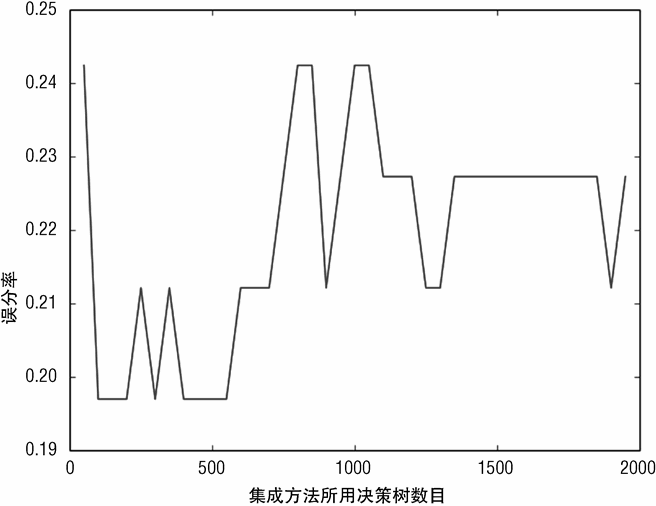
图 7-22 展示了随着决策树数目的增加,随机森林方法性能是如何改善的。随着决策树的增加,曲线通常是下降的。随着决策树的增加,改善的比率也在减少,当曲线达到最右边时,下降得已经相当缓慢了。
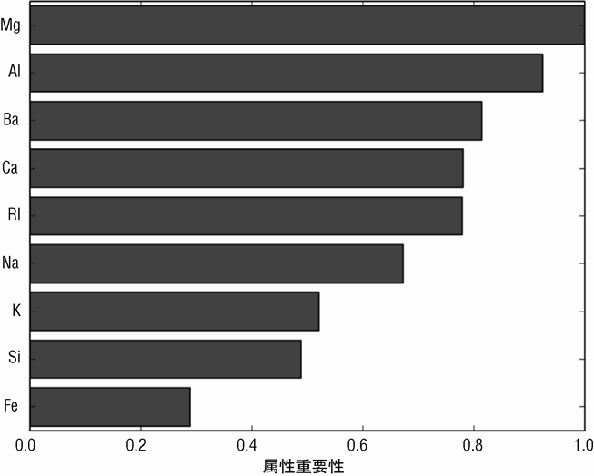
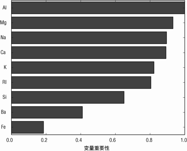
图 7-23 所示的条状图展示了随机森林所用属性的相对重要性排名。条状图说明有些属性对性能的贡献是相当的。这有些不同寻常。在很多情况下,属性的重要性经过前几个后会迅速下降。但在这个问题上,有几个属性具有相同的重要性。
7.5.3 用梯度提升法对玻璃进行分类
代码清单 7-9 除了一些小的差异外,其基本步骤与上节的使用随机森林对玻璃进行分类的过程基本一致。
代码清单 7-9 使用梯度提升法对玻璃进行分类 -glassGbm.py
__author__ = 'mike_bowles'
import urllib2
from math import sqrt, fabs, exp
import matplotlib.pyplot as plot
from sklearn.linear_model import enet_path
from sklearn.metrics import roc_auc_score, roc_curve, confusion_matrix
from sklearn.cross_validation import train_test_split
from sklearn import ensemble
import numpy
target_url = ("https://archive.ics.uci.edu/ml/machine-learning-databases/glass/glass.data")
data = urllib2.urlopen(target_url)
#arrange data into list for labels and list of lists for attributes
xList = []
for line in data:
#split on comma
row = line.strip().split(",")
xList.append(row)
glassNames = numpy.array(['RI', 'Na', 'Mg', 'Al', 'Si', 'K', 'Ca',
'Ba', 'Fe', 'Type'])
#Separate attributes and labels
xNum = []
labels = []
for row in xList:
labels.append(row.pop())
l = len(row)
#eliminate ID
attrRow = [float(row[i]) for i in range(1, l)]
xNum.append(attrRow)
#number of rows and columns in x matrix
nrows = len(xNum)
ncols = len(xNum[1])
#Labels are integers from 1 to 7 with no examples of 4.
#gb requires consecutive integers starting at 0
newLabels = []
labelSet = set(labels)
labelList = list(labelSet)
labelList.sort()
nlabels = len(labelList)
for l in labels:
index = labelList.index(l)
newLabels.append(index)
#Class populations:
#old label new label num of examples
#1 0 70
#2 1 76
#3 2 17
#5 3 13
#6 4 9
#7 5 29
#
#Drawing 30% test sample may not preserve population proportions
#stratified sampling by labels.
xTemp = [xNum[i] for i in range(nrows) if newLabels[i] == 0]
yTemp = [newLabels[i] for i in range(nrows) if newLabels[i] == 0]
xTrain, xTest, yTrain, yTest = train_test_split(xTemp, yTemp,
test_size=0.30, random_state=531)
for iLabel in range(1, len(labelList)):
#segregate x and y according to labels
xTemp = [xNum[i] for i in range(nrows) if newLabels[i] == iLabel]
yTemp = [newLabels[i] for i in range(nrows) if \
newLabels[i] == iLabel]
#form train and test sets on segregated subset of examples
xTrainTemp, xTestTemp, yTrainTemp, yTestTemp = train_test_split(
xTemp, yTemp, test_size=0.30, random_state=531)
#accumulate
xTrain = numpy.append(xTrain, xTrainTemp, axis=0)
xTest = numpy.append(xTest, xTestTemp, axis=0)
yTrain = numpy.append(yTrain, yTrainTemp, axis=0)
yTest = numpy.append(yTest, yTestTemp, axis=0)
#instantiate model
nEst = 500
depth = 3
learnRate = 0.003
maxFeatures = 3
subSamp = 0.5
glassGBMModel = ensemble.GradientBoostingClassifier(n_estimators=nEst,
max_depth=depth,learning_rate=learnRate,
max_features=maxFeatures,subsample=subSamp)
#train
glassGBMModel.fit(xTrain, yTrain)
# compute auc on test set as function of ensemble size
missClassError = []
missClassBest = 1.0
predictions = glassGBMModel.staged_decision_function(xTest)
for p in predictions:
missClass = 0
for i in range(len(p)):
listP = p[i].tolist()
if listP.index(max(listP)) != yTest[i]:
missClass += 1
missClass = float(missClass)/len(p)
missClassError.append(missClass)
#capture best predictions
if missClass < missClassBest:
missClassBest = missClass
pBest = p
idxBest = missClassError.index(min(missClassError))
#print best values
print("Best Missclassification Error" )
print(missClassBest)
print("Number of Trees for Best Missclassification Error")
print(idxBest)
#plot training deviance and test auc's vs number of trees in ensemble
missClassError = [100*mce for mce in missClassError]
plot.figure()
plot.plot(range(1, nEst + 1), glassGBMModel.train_score_,
label='Training Set Deviance', linestyle=":")
plot.plot(range(1, nEst + 1), missClassError, label='Test Set Error')
plot.legend(loc='upper right')
plot.xlabel('Number of Trees in Ensemble')
plot.ylabel('Deviance / Classification Error')
plot.show()
# Plot feature importance
featureImportance = glassGBMModel.feature_importances_
# normalize by max importance
featureImportance = featureImportance / featureImportance.max()
#plot variable importance
idxSorted = numpy.argsort(featureImportance)
barPos = numpy.arange(idxSorted.shape[0]) + .5
plot.barh(barPos, featureImportance[idxSorted], align='center')
plot.yticks(barPos, glassNames[idxSorted])
plot.xlabel('Variable Importance')
plot.show()
#generate confusion matrix for best prediction.
pBestList = pBest.tolist()
bestPrediction = [r.index(max(r)) for r in pBestList]
confusionMat = confusion_matrix(yTest, bestPrediction)
print('')
print("Confusion Matrix")
print(confusionMat)
# Printed Output:
#
# nEst = 500
# depth = 3
# learnRate = 0.003
# maxFeatures = None
# subSamp = 0.5
#
#
# Best Missclassification Error
# 0.242424242424
# Number of Trees for Best Missclassification Error
# 113
#
# Confusion Matrix
# [[19 1 0 0 0 1]
# [ 3 19 0 1 0 0]
# [ 4 1 0 0 1 0]
# [ 0 3 0 1 0 0]
# [ 0 0 0 0 3 0]
# [ 0 1 0 1 0 7]]
#
# For Gradient Boosting using Random Forest base learners
# nEst = 500
# depth = 3
# learnRate = 0.003
# maxFeatures = 3
# subSamp = 0.5
#
#
#
# Best Missclassification Error
# 0.227272727273
# Number of Trees for Best Missclassification Error
# 267
#
# Confusion Matrix
# [[20 1 0 0 0 0]
# [ 3 20 0 0 0 0]
# [ 3 3 0 0 0 0]
# [ 0 4 0 0 0 0]
# [ 0 0 0 0 3 0]
# [ 0 2 0 0 0 7]]
如前所述,在 GradientBoostingClassifier 类中可以使用迭代版本的梯度提升法,这样在梯度提升的训练过程中每一步都可以生成预测结果。
7.5.4 评估在梯度提升法中使用随机森林基学习器的好处
在代码的最后可以看到 max_features 分别设为 None 和 20 时,梯度提升法的预测结果。
第一个取值是指训练普通的决策树,就像最初提出梯度提升法算法的论文建议的那样。第二个取值是指将随机森林作为基学习器,在决策树的每个节点进行数据分割时不考虑所有的属性,只随机考虑 max_features 个属性。这实际上是梯度提升和随机森林两种方法的混合。
训练数据集的偏差和测试数据集上的误分类误差如图 7-24 所示。偏差展示了训练的过程。测试数据集的误分类误差用来确定模型是否过拟合。算法没有过拟合,但是在决策树数目达到 200 左右后,性能也不再提升,因此可以终止测试。
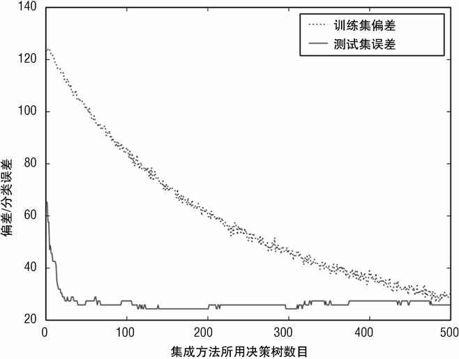
图 7-25 为梯度提升法中各属性的重要性排名。此图不太寻常,有相当多属性的重要性差不多。通常是有几个属性非常重要,然后后续属性的重要性迅速下降。
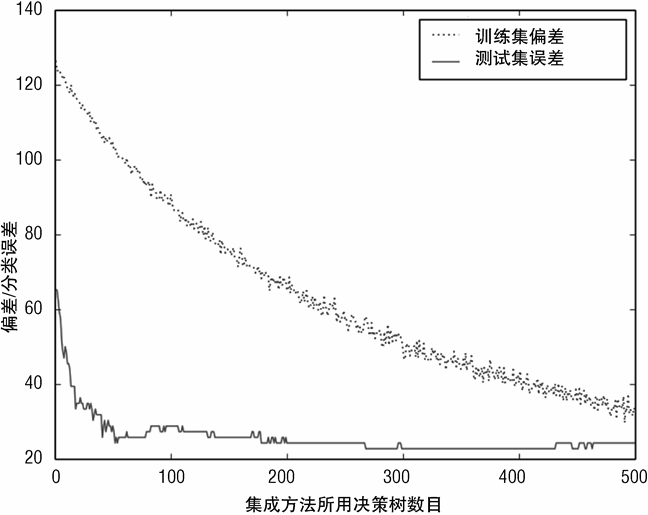
当 max_features 取值为 20 时,其训练数据偏差和测试数据误分类误差如图 7-26 所示,这时使用的是随机森林基学习器。这导致误分类率改善了大概 10%。但在图 7-26 中察觉不到,这种轻微的改善并不能改变图 7-26 中曲线的基本特征。

基于随机森林基学习器的梯度提升法所用属性的重要性排名如图 7-27 所示。此图各属性的排名与图 7-25 中的有些不同。有些属性都出现在两个排名的前五,但是有些属性在一个排名中出现在前五,但在另一个排名中却出现在最后。这两个图都显示了某些属性具有类似的重要,这可能是这两个排名有些不稳定的原因。


本书评论