Python机器学习——预测分析核心算法

自举集成（bootstrap aggregation 即 Bagging 算法）是由 Leo Breiman 提出的。该方法是从选取一个基学习器开始的，本书使用二元决策树作为基学习器。随着对此方法介绍的深入，可以看到其他机器学习算法也可以作为基学习器。二元决策树是合乎逻辑地选择，因为它可以对具有复杂决策边界的问题建模，但二元决策树性能表现很不稳定。这种不稳定性可以通过组合多个基于决策树的模型来克服。

6.2.1 Bagging 算法是如何工作的

自举集成算法使用叫作自举（bootstrap）的取样方法。自举取样通常用来从一个中等规模的数据集中产生取样统计。一个（非参）自举取样是从数据集放回式地随机选择元素（也就是说，自举取样可能会重复取出原始数据中的同一行数据）。自举集成从训练数据集中获得一系列的自举样本，然后针对每一个自举样本训练一个基学习器。对于回归问题，结果为基学习器的均值。对于分类问题，结果是从不同类别所占的百分比引申出来的各种类别的概率或均值。代码清单 6-4 展示了对本章开始介绍的合成数据问题如何应用Bagging 算法。

代码预留 30% 的数据作为测试数据，以代替交叉验证方法。参数 numTreesMax 决定集成方法包含的决策树的最大数目。代码建立模型是从第一个决策树开始，然后是前两个决策树、前三个决策树，以此类推，直到 numTreesMax 个决策树，可以看到预测的准确性与决策树数目之间的关系。代码将训练好的模型存入一个列表，并且存储了测试数据的预测值，这些预测值用于评估测试误差。代码画了两个图，一个展示了当集成方法增加决策树时，均方误差是如何变化的。另外一个图展示了第一个决策树的预测值、前 10 个决策树的平均预测值和前 20 个决策树的平均预测值的对比图。这个对比分析图与预测值曲线和实际标签值的对比图十分相似。

代码清单 6-4 自举集成算法 -simpleBagging.py

__author__ = 'mike-bowles'
import numpy
import matplotlib.pyplot as plot
from sklearn import tree
from sklearn.tree import DecisionTreeRegressor
from math import floor
import random
#Build a simple data set with y = x + random
nPoints = 1000
#x values for plotting
xPlot = [(float(i)/float(nPoints) - 0.5) for i in range(nPoints + 1)]
#x needs to be list of lists.
x = [[s] for s in xPlot]
#y (labels) has random noise added to x-value
#set seed
random.seed(1)
y = [s + random.normal(scale=0.1) for s in xPlot]
#take fixed test set 30% of sample
nSample = int(nPoints * 0.30)
idxTest = random.sample(range(nPoints), nSample)
idxTest.sort()
idxTrain = [idx for idx in range(nPoints) if not(idx in idxTest)]
#Define test and training attribute and label sets
xTrain = [x[r] for r in idxTrain]
xTest = [x[r] for r in idxTest]
yTrain = [y[r] for r in idxTrain]
yTest = [y[r] for r in idxTest]
#train a series of models on random subsets of the training data
#collect the models in a list and check error of composite as list grows
#maximum number of models to generate
numTreesMax = 20
#tree depth - typically at the high end
treeDepth = 1
#initialize a list to hold models
modelList = []
predList = []
#number of samples to draw for stochastic bagging
nBagSamples = int(len(xTrain) * 0.5)
for iTrees in range(numTreesMax):
idxBag = random.sample(range(len(xTrain)), nBagSamples)
xTrainBag = [xTrain[i] for i in idxBag]
yTrainBag = [yTrain[i] for i in idxBag]
modelList.append(DecisionTreeRegressor(max_depth=treeDepth))
modelList[-1].fit(xTrainBag, yTrainBag)
#make prediction with latest model and add to list of predictions
latestPrediction = modelList[-1].predict(xTest)
predList.append(list(latestPrediction))
#build cumulative prediction from first "n" models
mse = []
allPredictions = []
for iModels in range(len(modelList)):
#average first "iModels" of the predictions
prediction = []
for iPred in range(len(xTest)):
prediction.append(sum([predList[i][iPred] ＼
for i in range(iModels + 1)])/(iModels + 1))
allPredictions.append(prediction)
errors = [(yTest[i] - prediction[i]) for i in range(len(yTest))]
mse.append(sum([e * e for e in errors]) / len(yTest))
nModels = [i + 1 for i in range(len(modelList))]
plot.plot(nModels,mse)
plot.axis('tight')
plot.xlabel('Number of Models in Ensemble')
plot.ylabel('Mean Squared Error')
plot.ylim((0.0, max(mse)))
plot.show()
plotList = [0, 9, 19]
for iPlot in plotList:
plot.plot(xTest, allPredictions[iPlot])
plot.plot(xTest, yTest, linestyle="--")
plot.axis('tight')
plot.xlabel('x value')
plot.ylabel('Predictions')
plot.show()

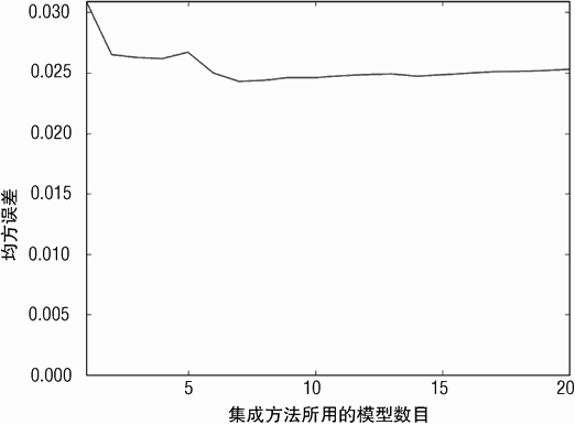
图 6-11 展示了当决策树数目增加时均方误差是如何变化的。误差在 0.025 左右稳定下来。这个结果并不好。添加的噪声标准差为 0.1。一个预测算法的最佳均方误差应该是这个标准差的平方，也就是 0.01。本章前面的单个二进制决策树就已经接近 0.01 了。为什么复杂的算法性能反倒下降？

Bagging 的性能 - 偏差与方差（bias vs.variance)

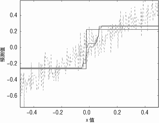
仔细观察图 6-12 会对这个问题提供些启示，其中有一个重要的关键点需要明确指出，这个关键点与其他问题也有关系。图 6-12 展示了单个决策树的预测结果、10 个决策树的预测结果、20 个决策树的预测结果。单个决策树的预测值很容易看清楚，因为只有一个“台阶”。10 个决策树和 20 个决策树的预测实际上叠加了一系列稍有不同的决策树，因此它们实际上是在单个决策树那个单一台阶的附近增加了一系列更精细的“台阶”。

多个决策树的台阶并不都在同一个点上，因为它们是基于不同的取样数据进行训练的，导致了分割点有一定的随机性。但随机性只会在分割点附近的小范围内带来轻微扰动。

因此，结果看起来变化并不大，因为所有的决策树对于应该在哪里进行分割是有大概共识的。

这里存在两种误差：偏差和方差。考虑用一条直线来拟合一个摆动的曲线。增加数据规模可以减少噪声对拟合数据的影响，但是再多的数据也不可能让直线完全匹配一个摆动的曲线。当更多的数据点加入时，并不能减少的误差叫作偏差（bias errors)。用深度为1 的决策树对合成数据拟合就会有偏差。所有的分割点都选在数据中心附近，因此对边缘数据的预测会影响模型的准确率。

深度为 1 的决策树的偏差来自于模型太简单了。Bagging 方法减少了模型之间的方差。

但是对深度为 1 的决策树的偏差错误则是平均不掉的。克服这个问题的方法就是增加决策树的深度。

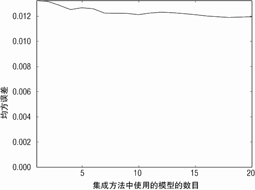
对应集成方法采用深度为 5 的决策树时，均方误差与决策树数目的关系图如图 6-13所示。当采用深度为 5 的决策树时，均方误差稍微小于 0.01（可能是由于噪声数据的随机性），明显性能要好于深度为 1 的决策树。

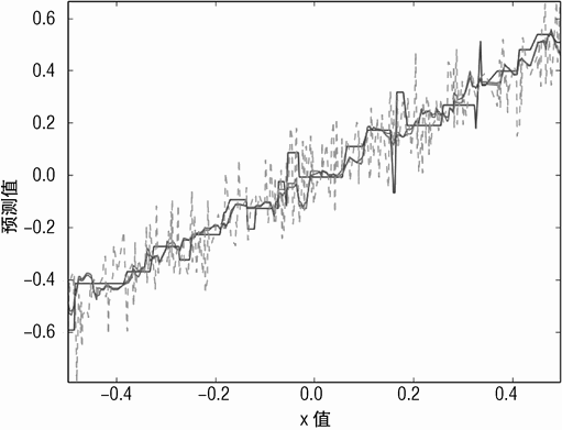
使用 1 个决策树、10 个决策树、20 个决策树的预测结果如图 6-14 所示。单个决策树的预测结果明显比其他的突出，因为它有几个尖锐的突出，这导致了严重的误差。换句话说，单个决策树有高的方差。其他单个的决策树毫无疑问具有相似的性能。但是当它们被平均时（采用集成方法），方差减少了；基于 Bagging 算法的预测曲线更光滑，更接近于真实值。

Bagging 算法如何解决多变量问题代码清单 6-5 展示了 Bagging 算法如何解决预测红酒口感问题。红酒口感例子展示了与合成数据问题一致的处理原则，如图 6-15 ～图 6-17 所示。这些图是通过设置不同的参数，运行代码清单 6-5 获得的。

代码清单 6-5 用 Bagging 算法预测红酒口感 -wineBagging.py

__author__ = 'mike-bowles'
import urllib2
import numpy
from sklearn import tree
from sklearn.tree import DecisionTreeRegressor
import random
from math import sqrt
import matplotlib.pyplot as plot
#read data into iterable
target_url = ("http://archive.ics.uci.edu/ml/machine-learning-databases/wine-quality/winequality-red.csv")
data = urllib2.urlopen(target_url)
xList = []
labels = []
names = []
firstLine = True
for line in data:
if firstLine:
names = line.strip().split(";")
firstLine = False
else:
#split on semi-colon
row = line.strip().split(";")
#put labels in separate array
labels.append(float(row[-1]))
#remove label from row
row.pop()
#convert row to floats
floatRow = [float(num) for num in row]
xList.append(floatRow)
nrows = len(xList)
ncols = len(xList[0])
#take fixed test set 30% of sample
random.seed(1)
nSample = int(nrows * 0.30)
idxTest = random.sample(range(nrows), nSample)
idxTest.sort()
idxTrain = [idx for idx in range(nrows) if not(idx in idxTest)]
#Define test and training attribute and label sets
xTrain = [xList[r] for r in idxTrain]
xTest = [xList[r] for r in idxTest]
yTrain = [labels[r] for r in idxTrain]
yTest = [labels[r] for r in idxTest]
#train a series of models on random subsets of the training data
#collect the models in a list and check error of composite as list grows
#maximum number of models to generate
numTreesMax = 30
#tree depth - typically at the high end
treeDepth = 1
#initialize a list to hold models
modelList = []
predList = []
#number of samples to draw for stochastic bagging
nBagSamples = int(len(xTrain) * 0.5)
for iTrees in range(numTreesMax):
idxBag = []
for i in range(nBagSamples):
idxBag.append(random.choice(range(len(xTrain))))
xTrainBag = [xTrain[i] for i in idxBag]
yTrainBag = [yTrain[i] for i in idxBag]
modelList.append(DecisionTreeRegressor(max_depth=treeDepth))
modelList[-1].fit(xTrainBag, yTrainBag)
#make prediction with latest model and add to list of predictions
latestPrediction = modelList[-1].predict(xTest)
predList.append(list(latestPrediction))
#build cumulative prediction from first "n" models
mse = []
allPredictions = []
for iModels in range(len(modelList)):
#average first "iModels" of the predictions
prediction = []
for iPred in range(len(xTest)):
prediction.append(sum([predList[i][iPred] ＼
for i in range(iModels + 1)])/(iModels + 1))
allPredictions.append(prediction)
errors = [(yTest[i] - prediction[i]) for i in range(len(yTest))]
mse.append(sum([e * e for e in errors]) / len(yTest))
nModels = [i + 1 for i in range(len(modelList))]
plot.plot(nModels,mse)
plot.axis('tight')
plot.xlabel('Number of Tree Models in Ensemble')
plot.ylabel('Mean Squared Error')
plot.ylim((0.0, max(mse)))
plot.show()
print('Minimum MSE')
print(min(mse))
#with treeDepth = 1
#Minimum MSE
#0.516236026081
#with treeDepth = 5
#Minimum MSE
#0.39815421341
#with treeDepth = 12 & numTreesMax = 100
#Minimum MSE
#0.350749027669

图 6-15 展示了在 Bagging 集成方法中包含更多决策树时，均方误差如何变化。基于树桩（stumps，深度为 1 的决策树）的集成方法相对于单个决策树在均方误差方面的改善可以忽略不计。与合成数据相比，红酒数据更加没有体现性能上的改善主要有以下几个原因：一方面红酒口感数据集边缘数据产生的误差更加显著，另外一方面变量（属性）之间相关性（相互作用）在红酒数据上更加突出。

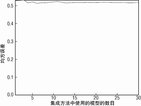
合成数据只有一个变量（属性），因此不存在属性之间的相互影响。红酒数据有多个属性，因此很可能属性的组合对预测的贡献要大于单独每个属性对预测的贡献和。“当你走路的时候被绊倒了，这个问题不大。如果你沿着悬崖走，问题也不严重。但是如果在沿着悬崖走的时候被绊倒了，这个问题可就严重了”（屋漏偏逢连夜雨）。上述两种可能性都要考虑。深度为 1 的决策树只能考虑单独的属性，没有考虑到属性之间相互影响的情况。

Bagging 算法为达到一定性能需要的决策树深度图 6-16 展示了决策树深度为 5 时，均方误差与决策树数目的变化关系。随着更多的决策树加入，Bagging 集成方法的性能有明显改善。最终的性能要远远好与深度为 1 的决策树。这种改善暗示了当加入更多的决策树时，性能会进一步提高。

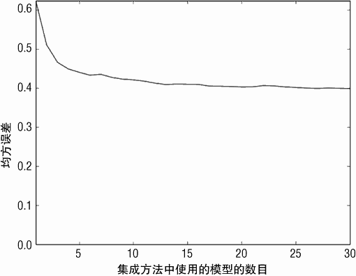
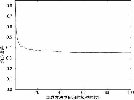
图 6-17 展示了决策树深度为 12 时，Bagging 集成方法的均方误差与决策树数目的关系。

不仅可以采用更深的决策树，含有更多的决策树数目也可以进一步提升 Bagging 集成方法的性能。图 6-17 展示的是运行三次中最低的均方误差。

6.2.2 Bagging 算法小结

本节见证了集成方法的第一个例子。Bagging 方法展示的二级层次架构对集成方法来讲很普遍。准确地说 Bagging 是第二层次的算法：它定义了一系列的子问题，每个子问题由基学习器来解决，最终预测结果取各个基学习器预测的平均值。Bagging 集成方法的这些子问题是从原始训练数据中采用自举取样产生的。Bagging 方法可以减少单个二元决策树的方差。为了保证效果，Bagging 方法采用的决策树需要具有足够的深度。

Bagging 方法可以作为集成方法的入门介绍，因为它比较简单，易于理解，而且易于证明它可以减少方差的特性。下面介绍的算法是梯度提升法（gradient boosting）和随机森林（random forests）。它们采用不同的方法进行集成，并且显示了优于 Bagging方法的特性。人们通常首先尝试梯度提升法或者随机森林，但是不常使用 Bagging。