
6.3 梯度提升法(Gradient Boosting)
梯度提升法由斯坦福教授 Jerome Frideman 提出,他也提出坐标下降法来解决ElasticNet 问题(见第 4 章和第 5 章)。梯度提升法是基于决策树的集成方法,在不同标签上训练决策树,然后将其组合起来。对于回归问题,目标是最小化均方误差,每个后续的决策树是在前面决策树遗留的错误上进行训练。关于此算法的来源可以查看本章的参考文献。了解梯度提升法是如何工作的最简单的方法就是直接查看代码实现。
6.3.1 梯度提升法的基本原理
代码清单 6-6 展示了针对本章的合成数据问题如何应用梯度提升法。代码的前面部分是生成合成数据集。
代码清单 6-6 简单问题使用梯度提升法 -simpleGBM.py
__author__ = 'mike-bowles'
import numpy
import matplotlib.pyplot as plot
from sklearn import tree
from sklearn.tree import DecisionTreeRegressor
from math import floor
import random
#Build a simple data set with y = x + random
nPoints = 1000
#x values for plotting
xPlot = [(float(i)/float(nPoints) - 0.5) for i in range(nPoints + 1)]
#x needs to be list of lists.
x = [[s] for s in xPlot]
#y (labels) has random noise added to x-value
#set seed
numpy.random.seed(1)
y = [s + numpy.random.normal(scale=0.1) for s in xPlot]
#take fixed test set 30% of sample
nSample = int(nPoints * 0.30)
idxTest = random.sample(range(nPoints), nSample)
idxTest.sort()
idxTrain = [idx for idx in range(nPoints) if not(idx in idxTest)]
#Define test and training attribute and label sets
xTrain = [x[r] for r in idxTrain]
xTest = [x[r] for r in idxTest]
yTrain = [y[r] for r in idxTrain]
yTest = [y[r] for r in idxTest]
#train a series of models on random subsets of the training data
#collect the models in a list and check error of composite as list grows
#maximum number of models to generate
numTreesMax = 30
#tree depth - typically at the high end
treeDepth = 5
#initialize a list to hold models
modelList = []
predList = []
eps = 0.3
#initialize residuals to be the labels y
residuals = list(yTrain)
for iTrees in range(numTreesMax):
modelList.append(DecisionTreeRegressor(max_depth=treeDepth))
modelList[-1].fit(xTrain, residuals)
#make prediction with latest model and add to list of predictions
latestInSamplePrediction = modelList[-1].predict(xTrain)
#use new predictions to update residuals
residuals = [residuals[i] - eps * latestInSamplePrediction[i] \
for i in range(len(residuals))]
latestOutSamplePrediction = modelList[-1].predict(xTest)
predList.append(list(latestOutSamplePrediction))
#build cumulative prediction from first "n" models
mse = []
allPredictions = []
for iModels in range(len(modelList)):
#add the first "iModels" of the predictions and multiply by eps
prediction = []
for iPred in range(len(xTest)):
prediction.append(sum([predList[i][iPred]
for i in range(iModels + 1)]) * eps)
allPredictions.append(prediction)
errors = [(yTest[i] - prediction[i]) for i in range(len(yTest))]
mse.append(sum([e * e for e in errors]) / len(yTest))
nModels = [i + 1 for i in range(len(modelList))]
plot.plot(nModels,mse)
plot.axis('tight')
plot.xlabel('Number of Models in Ensemble')
plot.ylabel('Mean Squared Error')
plot.ylim((0.0, max(mse)))
plot.show()
plotList = [0, 14, 29]
lineType = [':', '-.', '--']
plot.figure()
for i in range(len(plotList)):
iPlot = plotList[i]
textLegend = 'Prediction with ' + str(iPlot) + ' Trees'
plot.plot(xTest, allPredictions[iPlot], label = textLegend,
linestyle = lineType[i])
plot.plot(xTest, yTest, label='True y Value', alpha=0.25)
plot.legend(bbox_to_anchor=(1,0.3))
plot.axis('tight')
plot.xlabel('x value')
plot.ylabel('Predictions')
plot.show()
梯度提升法参数设置
第一个与前面例子的不同之处就是单个决策树深度的设置。梯度提升法与 Bagging 和随机森林的不同之处在于它在减少方差的同时,还可以减少偏差。梯度提升法的特性就是它在树桩(深度为 1 的决策树)决策树的情况下,也可以获得同更深的决策树一样低的均方误差值。对于梯度提升法,只有属性之间有强烈的相互影响的情况下,才需要考虑增加决策树的深度。随着决策树深度的增加,性能获得了改善实际上可以作为判断属性之间是否存在相互影响的方法。
另一个不同点就是变量 eps 的定义。这个变量在优化问题时用来控制步长。梯度提升法使用了梯度下降法,就像其他梯度下降算法一样,如果步长太大,优化过程就会发散而不是收敛。如果步长太小,则需要执行太多次迭代。本章后续会讨论如何调整步长,即 eps 值。
下一段不太熟悉的代码就是关于变量残差(residuals)的定义。术语残差通常用于表示预测误差(在这里是:观测值减去预测值)。梯度提升法会对标签的预测值进行一系列精确化。沿着梯度下降的方向,每走一步,残差都会重新计算。在开始阶段,梯度提升法将初始化预测值为空(null)或 0,因此残差等于观测值。
梯度提升法如何通过迭代获得预测模型
对 iTrees 的循环是以用属性值训练一个决策树开始的,但是用残差代替标签进行训练。
只有第一轮是用原始的标签来训练数据的。后续的循环都是用训练产生的预测值,然后用残差减去(eps* 预测值)作为目标结果进行训练。如前文提到的,残差减去的相当于梯度下降的值。乘以一个步长控制参数 eps 就是为了保证迭代过程的收敛。代码使用固定的预留数据集(测试数据)来测量性能,并绘制了均方误差与决策树数目的关系图以及预测值与单一属性值的关系图。
6.3.2 获取梯度提升法的最佳性能
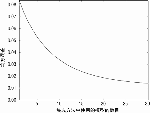
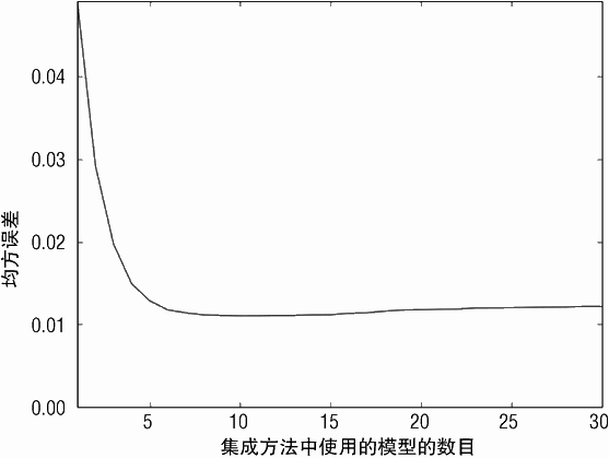
图 6-18 和图 6-19 展示了均方误差与决策树数目的关系图,预测值与属性值的关系图,决策树深度为 1,eps=0.1。图 6-18 展示了均方误差平滑下降,在训练了 30 个决策树的情况下,大概达到 0.014。均方误差曲线向下,说明随着决策树的增加,其值会持续下降。
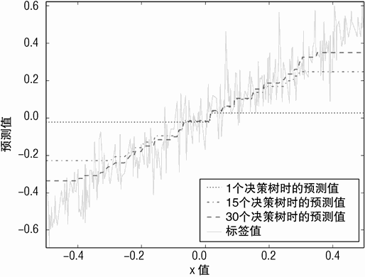
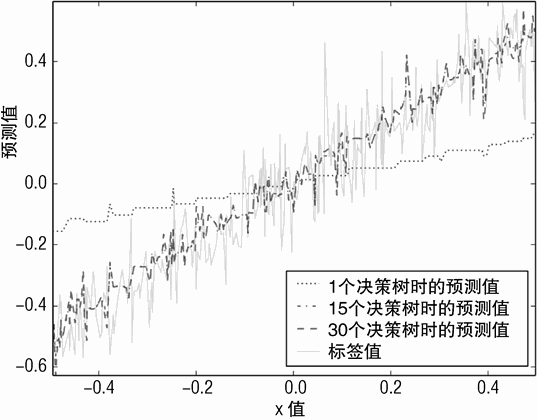
训练 15 个决策树、训练 30 个决策树。训练一个决策树的模型就像是我们在决策树介绍章节见到过的决策树模型的减弱版本。它实际上是一个深度为 1 的决策树,基于标签进行训练,然后再乘以 0.1(eps 的值)。当模型使用 10 个决策树时,有趣的现象出现了。模型实现了对正确答案(一个 45 度角的直线)很好的逼近。使用 10 个决策树的模型大概可以正确预测一半的边界,其右边、左边的预测值为常数。使用 30 个决策树的模型在每个数据的边界都实现了很好的逼近。在这一点上与采用树桩(stumps)决策树的 Bagging方法有很大区别。
图 6-19 梯度提升法,预测值与属性值的关系(eps=0.1, 决策树深度为 1)
Bagging 方法不能改善偏差(bias error),这是由浅决策树固有特性决定的。梯度提升法以同样的方式开始,但是随着它开始减少过程中产生的错误,它开始更关注犯错误的区域。在会发生错误的地方设立分割点。这个过程使得不需要加深决策树的深度,就可以获得很好的逼近。
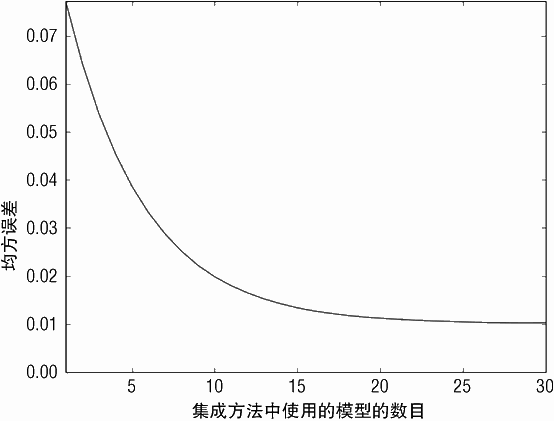
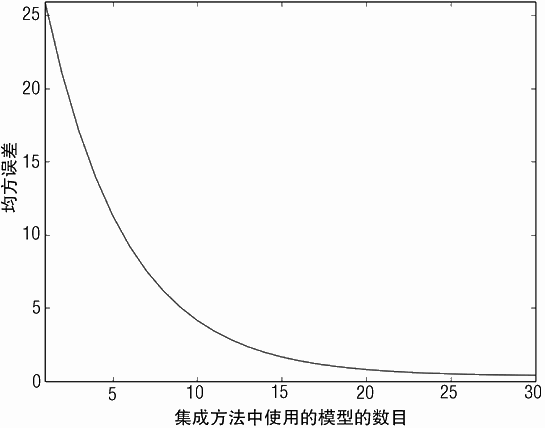
当控制训练的参数变化时会发生什么?当决策树的深度为 5 时发生的变化如图 6-20 和图 6-21 所示。当决策树的数目增加时,均方误差会平滑下降,如图 6-20 所示。当训练30 个深度为 5 的决策树时,均方误差非常接近完美值(0.01)。图中没有显示训练时间。
训练时,决策树的每一层大约花费相同的时间。在每一层,所有可能的分割点根据均方误差进行比较。因此深度为5的决策树所需时间是5个深度为1的决策树所需时间的5倍。
通过比较可知, 150 个深度为 1 的决策树的性能相当于 30 个深度为 5 的决策树。
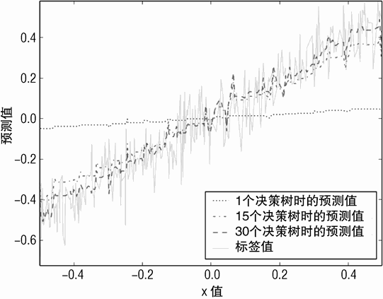
决策树深度对梯度提升方法的影响如图 6-21 所示。即使只采用了单独一个决策树,其预测值在整个属性值区间也显示了一些变化。基于 15 个决策树的模型和 30 个决策树的模型在数据的边界仍然有一定的误差。
图 6-22 和图 6-23 展示了增加步长参数 eps 会发生什么。图 6-22 展示了步长(eps)
太大会有什么特性。均方误差随着决策树数目的增加而急剧下降,然后又缓慢增加。其最小值是在图的左边,接近三分之一的地方。可以调整 eps 的值,使均方误差最小值在或者接近图的右侧,这样通常可以获得更佳的性能。
如图 6-23 所示,预测值作为属性值的函数 eps 为 0.3 的版本要比 eps 为 0.1 的两个版本(深度为 1 的决策树、深度为 5 的决策树)沿 45% 的直线显示了更多分散的突起。总的来看,深度为 1 的决策树显示了最佳的性能。这说明训练更多的决策树,会进一步改善模型在数据边界上的性能,从而获得梯度提升的最佳性能。
6.3.3 针对多变量问题的梯度提升法
代码清单 6-7 展示了如何使用梯度提升法来预测红酒口感。除了使用红酒数据集作为输入外,此代码与用于合成数据的代码十分相似。
代码清单 6-7 使用梯度提升法预测红酒口感 -wineGBM.py
__author__ = 'mike-bowles'
import urllib2
import numpy
from sklearn import tree
from sklearn.tree import DecisionTreeRegressor
import random
from math import sqrt
import matplotlib.pyplot as plot
#read data into iterable
target_url = "http://archive.ics.uci.edu/ml/machine-learning-databases/wine-quality/winequality-red.csv")
data = urllib2.urlopen(target_url)
xList = []
labels = []
names = []
firstLine = True
for line in data:
if firstLine:
names = line.strip().split(";")
firstLine = False
else:
#split on semi-colon
row = line.strip().split(";")
#put labels in separate array
labels.append(float(row[-1]))
#remove label from row
row.pop()
#convert row to floats
floatRow = [float(num) for num in row]
xList.append(floatRow)
nrows = len(xList)
ncols = len(xList[0])
#take fixed test set 30% of sample
nSample = int(nrows * 0.30)
idxTest = random.sample(range(nrows), nSample)
idxTest.sort()
idxTrain = [idx for idx in range(nrows) if not(idx in idxTest)]
#Define test and training attribute and label sets
xTrain = [xList[r] for r in idxTrain]
xTest = [xList[r] for r in idxTest]
yTrain = [labels[r] for r in idxTrain]
yTest = [labels[r] for r in idxTest]
#train a series of models on random subsets of the training data
#collect the models in a list and check error of composite as list grows
#maximum number of models to generate
numTreesMax = 30
#tree depth - typically at the high end
treeDepth = 5
#initialize a list to hold models
modelList = []
predList = []
eps = 0.1
#initialize residuals to be the labels y
residuals = list(yTrain)
for iTrees in range(numTreesMax):
modelList.append(DecisionTreeRegressor(max_depth=treeDepth))
modelList[-1].fit(xTrain, residuals)
#make prediction with latest model and add to list of predictions
latestInSamplePrediction = modelList[-1].predict(xTrain)
#use new predictions to update residuals
residuals = [residuals[i] - eps * latestInSamplePrediction[i] \
for i in range(len(residuals))]
latestOutSamplePrediction = modelList[-1].predict(xTest)
predList.append(list(latestOutSamplePrediction))
#build cumulative prediction from first "n" models
mse = []
allPredictions = []
for iModels in range(len(modelList)):
#add the first "iModels" of the predictions and multiply by eps
prediction = []
for iPred in range(len(xTest)):
prediction.append(sum([predList[i][iPred]
for i in range(iModels + 1)]) * eps)
allPredictions.append(prediction)
errors = [(yTest[i] - prediction[i]) for i in range(len(yTest))]
mse.append(sum([e * e for e in errors]) / len(yTest))
nModels = [i + 1 for i in range(len(modelList))]
plot.plot(nModels,mse)
plot.axis('tight')
plot.xlabel('Number of Trees in Ensemble')
plot.ylabel('Mean Squared Error')
plot.ylim((0.0, max(mse)))
plot.show()
print('Minimum MSE')
print(min(mse))
#printed output
#Minimum MSE
#0.405031864814
选择的参数为:30 个深度为 5 决策树,eps=0.1。这个参数集产生的均方误差大致为 0.4。
对于同样的问题,此方法大概比 Bagging 的方法差 10%。可以尝试调整:决策树的数目、eps 步长和决策树的深度来看看是否可以获得更佳的性能。
均方误差与决策树数目的关系曲线在右边相当平坦,如图 6-24 所示。通过增加决策树的数目还是可能获得性能上的改善的。另外一个可能“压榨”性能的方法就是微调步长或决策树的深度。
6.3.4 梯度提升方法的小结
本节介绍了如何使用梯度提升方法、如何调整参数获得最佳性能,以及步长、决策树深度、决策树数目对性能的影响。还介绍了梯度提升法是如何避免偏差的,这个是Bagging 方法采用浅决策树时会遇到的问题。Bagging 和梯度提升法在工作原理上的根本差异在于梯度提升法持续监测自己的累积误差,然后使用残差进行后续训练。这种根本差异也解释了为什么当问题属性之间存在强的相互依赖、相互作用时,梯度提升法只需要调整决策树的深度。


本书评论