
3.4 模型与数据的均衡
本节使用最小二乘法(OLS)来说明几个问题。首先,它展示为什么 OLS 有时会对问题过拟合。过拟合是指训练数据和测试数据上的错误存在显著差异,比如上一节的OLS 用于解决岩石 - 水雷分类问题。其次,我们将引入 2 种方法来解决 OLS 的过拟合。
这些方法会培养你的直觉,为第 4 章提到的惩罚线性回归方法做铺垫。此外,克服过拟合问题的方法在许多现代机器学习算法中都会用到。现代算法往往会产生大量不同复杂度的模型,然后基于样本外数据的性能来权衡模型复杂度、问题复杂度以及数据集丰富程度,最终决定使用哪个模型。该过程会在后续重复使用。
普通的最小二乘法作为一个原型很好地展示了机器学习算法的方方面面。它是一个有监督的学习算法,包括训练过程以及测试过程。在某些情况下可能会过拟合。最小二乘法与其他现代的函数逼近算法都存在一些共性。然而,与现代机器学习算法相比,OLS 少一个重要特点。在原始公式中(最熟悉的公式),当过拟合发生时,没有办法阻止学习过程。这就像让汽车全速前进(当道路宽敞时很好,在紧急情况下就会有问题)。
幸运的是,有大量的工作都在改进最小二乘法,尽管最小二乘法距离当时发明它的高斯和勒让德已经过去了 200 年。本节引入 2 种方法来调整普通最小二乘法的瓶颈:前向逐步回归和岭回归。
3.4.1 通过权衡问题复杂度、模型复杂度以及数据集规模来选择模型
下面一些例子将介绍现代机器学习算法是如何进行调整来更好地拟合问题和数据集。
第一个例子是对最小二乘法进行修改,被称作前向逐步回归方法。具体工作过程如下:
回忆下公式 3-1 以及公式 3-2 定义要解决的问题(这里对应公式 3-10 以及公式 3-11),向量 Y 包含标签,矩阵 X 包含用于预测标签的属性。
如果这是一个回归问题,那么 Y 是包含实数的列向量,线性问题是找到一个权重向量β 以及一个标量 β₀(参照公式 3-12)。
线性模型的目标是选择 β 以更好地逼近 Y(参照公式 3-13)。
如果 X 的列数等于 X 的行数,并且 X 不同列之间是相互独立的(不存在相互之间的线性关系),那么 X 可以求逆,符号~可以替换为 =。得到的向量 β 会更精确地拟合标签,看起来很好但不正确。问题在于出现了过拟合(过拟合是指在训练数据上预测效果很好但在新数据上不能复制)。对于真实问题,这并不是一个好的结果。过拟合的根源在于 X 中有太多的列。答案可能是去掉 X 中的一些列。然而去掉一些列又转化为去掉多少列以及哪几列应该去掉的问题。这种蛮力的方法也被称作最佳子集选择。
3.4.2 使用前向逐步回归来控制过拟合
下面代码简要勾勒了最佳子集选择算法的过程。
基本想法是在列的个数上增加一个约束(假设为 nCol),然后从 X 的所有列中抽取特定个数的列构成数据集,在上边执行最小二乘法,遍历所有列的组合(列数为 nCol),找到在测试集上取得最佳效果的 nCol 值;增加 nCol 值,重复上述过程。以上过程产生最佳的一列子集、两列子集一直到所有列子集(对应矩阵 X)。对于每个子集同样有一个性能与之对应。下一步决定在部署时是使用一列子集版本、两列子集版本,还是其他版本。到这就简单了,直接选择错误率最低的版本。
Initialize: Out_of_sample_error = NULL
Break X and Y into test and training sets
for i in range(number of columns in X):
for each subset of X having i+1 columns:
fit ordinary least squares model
Out_of_sample_error.append(least error amoung subsets containing
i+1 columns)
Pick the subset corresponding to least overall error
最佳子集选择存在的一个问题是该算法需要大量计算,即使属性不多的情况下(属性数对应 X 的列数),计算量也非常巨大。例如,10 个属性对应于 210=1000 个子集。有几种方法可以避免这种情况。下面的代码展示了前向逐步回归的过程。前向逐步回归的想法是从 1 列子集开始,找到效果最佳的那一列属性,接着寻找与其组合与效果最佳的第 2列属性,而不是评估所有的 2 列子集。前向逐步回归的伪代码如下。
Initialize: ColumnList = NULL
Out-of-sample-error = NULL
Break X and Y into test and training sets
For number of column in X:
For each trialColumn (column not in ColumnList):
Build submatrix of X using ColumnList + trialColumn
Train OLS on submatrix and store RSS Error on test data
ColumnList.append(trialColumn that minimizes RSS Error)
Out-of-sample-error.append(minimum RSS Error)
最佳子集选择以及前向逐步回归过程基本类似。它们训练一系列的模型(列数为 1 训练几个,列数为 2 训练几个,等等)。这种方法产生了参数化的模型族(所有线性回归以列数作为参数)。这些模型在复杂度上存在差异,最后的模型通过在预留样本上计算错误进行选择。
代码清单 3-3 为在红酒数据集上实现的前向逐步回归的 Python 代码。
代码清单 3-3 前向逐步回归:红酒品质数据 -fwdStepwiseWine.py
import numpy
from sklearn import datasets, linear_model
from math import sqrt
import matplotlib.pyplot as plt
def xattrSelect(x, idxSet):
#takes X matrix as list of list and returns subset containing
#columns in idxSet
xOut = []
for row in x:
xOut.append([row[i] for i in idxSet])
return(xOut)
#read data into iterable
target_url = ("http://archive.ics.uci.edu/ml/machine-learningdatabases/"
"wine-quality/winequality-red.csv")
data = urllib2.urlopen(target_url)
xList = []
labels = []
names = []
firstLine = True
for line in data:
if firstLine:
names = line.strip().split(";")
firstLine = False
else:
#split on semi-colon
row = line.strip().split(";")
#put labels in separate array
labels.append(float(row[-1]))
#remove label from row
row.pop()
#convert row to floats
floatRow = [float(num) for num in row]
xList.append(floatRow)
#divide attributes and labels into training and test sets
indices = range(len(xList))
xListTest = [xList[i] for i in indices if i%3 == 0 ]
xListTrain = [xList[i] for i in indices if i%3 != 0 ]
labelsTest = [labels[i] for i in indices if i%3 == 0]
labelsTrain = [labels[i] for i in indices if i%3 != 0]
#build list of attributes one-at-a-time - starting with empty
attributeList = []
index = range(len(xList[1]))
indexSet = set(index)
indexSeq = []
oosError = []
for i in index:
attSet = set(attributeList)
#attributes not in list already
attTrySet = indexSet - attSet
#form into list
attTry = [ii for ii in attTrySet]
errorList = []
attTemp = []
#try each attribute not in set to see which
#one gives least oos error
for iTry in attTry:
attTemp = [] + attributeList
attTemp.append(iTry)
#use attTemp to form training and testing sub matrices
#as list of lists
xTrainTemp = xattrSelect(xListTrain, attTemp)
xTestTemp = xattrSelect(xListTest, attTemp)
#form into numpy arrays
xTrain = numpy.array(xTrainTemp)
yTrain = numpy.array(labelsTrain)
xTest = numpy.array(xTestTemp)
yTest = numpy.array(labelsTest)
#use sci-kit learn linear regression
wineQModel = linear_model.LinearRegression()
wineQModel.fit(xTrain,yTrain)
#use trained model to generate prediction and calculate rmsError
rmsError = numpy.linalg.norm((yTest-wineQModel.predict(xTest)),
2)/sqrt(len(yTest))
errorList.append(rmsError)
attTemp = []
iBest = numpy.argmin(errorList)
attributeList.append(attTry[iBest])
oosError.append(errorList[iBest])
print("Out of sample error versus attribute set size" )
print(oosError)
print("\n" + "Best attribute indices")
print(attributeList)
namesList = [names[i] for i in attributeList]
print("\n" + "Best attribute names")
print(namesList)
#Plot error versus number of attributes
x = range(len(oosError))
plt.plot(x, oosError, 'k')
plt.xlabel('Number of Attributes')
plt.ylabel('Error (RMS)')
plt.show()
#Plot histogram of out of sample errors for best number of attributes
#Identify index corresponding to min value,
#retrain with the corresponding attributes
#Use resulting model to predict against out of sample data.
#Plot errors (aka residuals)
indexBest = oosError.index(min(oosError))
attributesBest = attributeList[1:(indexBest+1)]
#Define column-wise subsets of xListTrain and xListTest
#and convert to numpy
xTrainTemp = xattrSelect(xListTrain, attributesBest)
xTestTemp = xattrSelect(xListTest, attributesBest)
xTrain = numpy.array(xTrainTemp); xTest = numpy.array(xTestTemp)
#train and plot error histogram
wineQModel = linear_model.LinearRegression()
wineQModel.fit(xTrain,yTrain)
errorVector = yTest-wineQModel.predict(xTest)
plt.hist(errorVector)
plt.xlabel("Bin Boundaries")
plt.ylabel("Counts")
plt.show()
#scatter plot of actual versus predicted
plt.scatter(wineQModel.predict(xTest), yTest, s=100, alpha=0.10)
plt.xlabel('Predicted Taste Score')
plt.ylabel('Actual Taste Score')
plt.show()
上面的代码清单包含一个函数用于从 X 矩阵中抽取选择的列(对应于 Python 的列表list,该列表的每个元素也是一个列表)。然后该函数将 X 矩阵与标签向量划分为训练集和测试集。之后,代码完成前面描述的算法。算法的遍历从属性的一个子集开始。第一遍时,该子集为空。对于后续的遍历,该子集包含上一次遍历选择的属性。每一次遍历都会选择一个新的属性添加到属性子集中。待添加的属性是通过对每一个非包含的属性进行测试:
选择添加属性以后性能提高最多的属性。每一个属性被加入属性子集以后,使用普通的最小二乘法来拟合模型。对每一个测试属性,在预留样本上评估性能。产生最佳根损失(RSS)的属性被加入属性集,关联的 RSS 错误也会进行计算。
图 3-13 为 RMSE 与用于回归的属性个数之间的函数关系。在 9 个属性全部包含进来以前,错误一直在降低,然后增加。
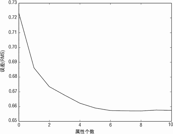
代码清单 3-4 为前向逐步回归方法应用于酒品质量预测的数值输出。
代码清单 3-4 前向逐步回归的输出 -fwdStepwiseWineOutput.txt
Out of sample error versus attribute set size
[0.7234259255116281, 0.68609931528371915, 0.67343650334202809,
0.66770332138977984, 0.66225585685222743, 0.65900047541546247,
0.65727172061430772, 0.65709058062076986, 0.65699930964461406,
0.65758189400434675, 0.65739098690113373]
Best attribute indices
[10, 1, 9, 4, 6, 8, 5, 3, 2, 7, 0]
Best attribute names
['"alcohol"', '"volatile acidity"', '"sulphates"', '"chlorides"',
'"total sulfur dioxide"', '"pH"', '"free sulfur dioxide"',
'"residual sugar"', '"citric acid"', '"density"', '"fixed acidity"']
第一个列表(python 的 list 对象)展示了 RSS 错误。错误一直降低,直到将第 10 个元素加入列表,然后错误变高。关联的列索引在后一个列表中给出。最后的列表给出了关联属性的名称(列名)。
3.4.3 评估并理解你的预测模型
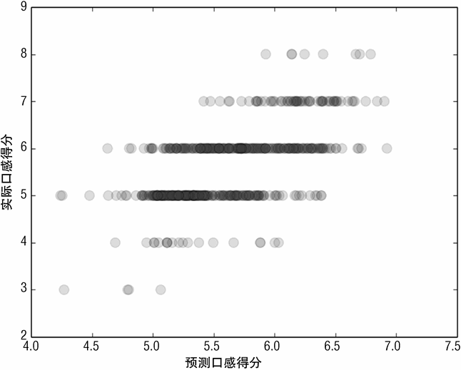
其他几个图对于理解一个学习好的算法性能非常有帮助,这些图指出了性能提升的途径。图 3-14 为测试集上每个点的实际标签值与预测标签值的散点图。在理想情况下,图 3-14中的所有点会分布在 45 度线上,这条线上的真正标签与预测标签是相等的。因为真正得分是整数,所以散点图分布在水平方向上。如果真正标签分布在少量的数值上,将每个数据点绘制成半透明状会很有用,一个区域的颜色深度就能反映点的堆积程度。对得分在 5和 6 上的实际酒品的预测结果非常好。对更极端的值,系统预测效果也不好。一般来讲,机器学习算法对边缘数据的预测效果并不好。
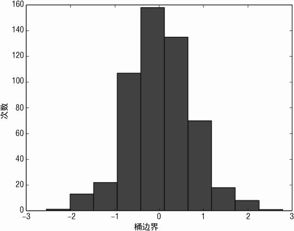
图 3-15 为前向逐步预测算法对酒品预测的错误直方图。有时错误直方图会有 2 个甚至多个离散的波峰,比如在最右边或者最左边有一个小的波峰。在这种情况下,可以继续寻找错误中不同波峰的解释,添加能够辨识归类的新属性来降低预测错误。
对于上面的输出结果要记住以下几点。首先,重新回顾一下整个学习过程,这里过程是指训练一组模型(在本例中,模型对应于基于 X 的列子集的普通线性回归)。这一系列模型进行了参数化(本例中,通过线性模型中的属性个数进行区分)。最终选择的模型在样本外的错误最小。解决方案中引入的属性个数称作复杂度参数。复杂度更高的模型会有更多自由参数,相对于低复杂度的模型更容易对数据产生过拟合。
另外注意到属性已经根据其对预测的重要性进行了排序。在包含列编号的 List 以及属性名的 List 中,第一个元素是第一个选择的属性,第二个元素是第二个选择的属性,以此类推。用到的属性按顺序排列。这是机器学习任务中一个很重要并且必需的特征。
早期机器学习任务大部分都包括寻找(或者构建)用于构建预测的最佳属性集。而能够对属性进行排序的算法对于上述任务非常有帮助。本书中介绍的其他算法也具备本特点。
最后一点是挑选模型。模型越复杂,泛化能力越差。在同等情况下,倾向于选择不太复杂的模型。前面例子表明从第 9 个模型到第 10 个模型的性能下降幅度很小(只在第 4位有变化)。最佳经验是如果属性添加后带来的性能提升只达到小数点后第 4 位,那么保守起见,可以将这样的属性移除掉。
3.4.4 通过惩罚回归系数来控制过拟合——岭回归
本节描述了另外一种通过修改最小二乘法来控制模型复杂度从而避免过拟合的方法。
这也是第一次介绍惩罚线性回归方法。第 4 章会更详细地介绍。
普通最小二乘法的目标是找到能够满足公式 3-14 的标量 β₀ 以及向量 β。
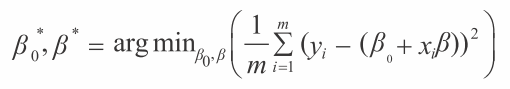
符号 argmin 是指“能够最小化表达式的 β₀ 以及 β”。系数 β₀* 以及 β* 是最小二乘法的解。
最佳子集回归以及前向逐步回归通过限制使用的属性个数来控制回归的复杂度。另外一种方法称作惩罚系数回归。惩罚系数回归是使系数变小,而不是将其中一些系数设为 0。一种惩罚线性回归的方法被称作岭回归。岭回归问题的定义见公式 3-15。
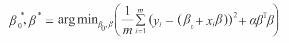
公式 3-15 以及普通最小二乘法(见公式 3-14)的差别在 αβTβ 项上。βTβ 项是β(系数向量)的欧几里得范数的平方。变量 β 是这类问题的复杂度参数。如果 α = 0,问题变为普通最小二乘法。如果 α 变大,β(系数的瓶阀)接近于 0,那么通过常数项 β₀就可以预测标签 yi。
scikit-learn包给出了岭回归的实现。代码清单3-5为使用岭回归来解决红酒口感回归问题的代码。
代码清单 3-5 使用岭回归预测红酒口感 -ridgeWine.py
__author__ = 'mike-bowles'
β β
import urllib2
import numpy
from sklearn import datasets, linear_model
from math import sqrt
import matplotlib.pyplot as plt
#read data into iterable
target_url = ("http://archive.ics.uci.edu/ml/machine-learningdatabases/"
"wine-quality/winequality-red.csv")
data = urllib2.urlopen(target_url)
xList = []
labels = []
names = []
firstLine = True
for line in data:
if firstLine:
names = line.strip().split(";")
firstLine = False
else:
#split on semi-colon
row = line.strip().split(";")
#put labels in separate array
labels.append(float(row[-1]))
#remove label from row
row.pop()
#convert row to floats
floatRow = [float(num) for num in row]
xList.append(floatRow)
#divide attributes and labels into training and test sets
indices = range(len(xList))
xListTest = [xList[i] for i in indices if i%3 == 0 ]
xListTrain = [xList[i] for i in indices if i%3 != 0 ]
labelsTest = [labels[i] for i in indices if i%3 == 0]
labelsTrain = [labels[i] for i in indices if i%3 != 0]
xTrain = numpy.array(xListTrain); yTrain = numpy.array(labelsTrain)
xTest = numpy.array(xListTest); yTest = numpy.array(labelsTest)
alphaList = [0.1**i for i in [0,1, 2, 3, 4, 5, 6]]
rmsError = []
for alph in alphaList:
wineRidgeModel = linear_model.Ridge(alpha=alph)
wineRidgeModel.fit(xTrain, yTrain)
rmsError.append(numpy.linalg.norm((yTest-wineRidgeModel.predict(
xTest)), 2)/sqrt(len(yTest)))
print("RMS Error alpha")
for i in range(len(rmsError)):
print(rmsError[i], alphaList[i])
#plot curve of out-of-sample error versus alpha
x = range(len(rmsError))
plt.plot(x, rmsError, 'k')
plt.xlabel('-log(alpha)')
plt.ylabel('Error (RMS)')
plt.show()
#Plot histogram of out of sample errors for best alpha value and
#scatter plot of actual versus predicted
#Identify index corresponding to min value, retrain with
#the corresponding value of alpha
#Use resulting model to predict against out of sample data.
#Plot errors (aka residuals)
indexBest = rmsError.index(min(rmsError))
alph = alphaList[indexBest]
wineRidgeModel = linear_model.Ridge(alpha=alph)
wineRidgeModel.fit(xTrain, yTrain)
errorVector = yTest-wineRidgeModel.predict(xTest)
plt.hist(errorVector)
plt.xlabel("Bin Boundaries")
plt.ylabel("Counts")
plt.show()
plt.scatter(wineRidgeModel.predict(xTest), yTest, s=100, alpha=0.10)
plt.xlabel('Predicted Taste Score')
plt.ylabel('Actual Taste Score')
plt.show()
回忆一下前向逐步回归算法生成了一系列不同的模型,第一个模型只包含一个属性,第二个模型包含两个属性,等等,直到最后的模型包含所有属性。岭回归代码也包含一系列的模型。岭回归通过不同的 α 值来控制模型数量,而不是通过属性个数来控制。α 参数决定了对 β 的惩罚力度。α 的一系列值按照 10 的倍数递减。一般来讲,你希望 α 按照指数级进行递减,并不是按照一个固定的增量。α 的取值范围一般要设置得足够宽,往往需要通过实验来确定。
图 3-16 为 RMSE 与岭回归的复杂度参数 α 的对应关系。参数按照从左到右、从大到小排列。传统习惯是一般在左边绘制简单模型,在右边绘制复杂模型。图 3-16 显示了与逐步前向回归类似的特点。错误几乎是一样的,但前向逐步回归的错误相比来说更大一些。
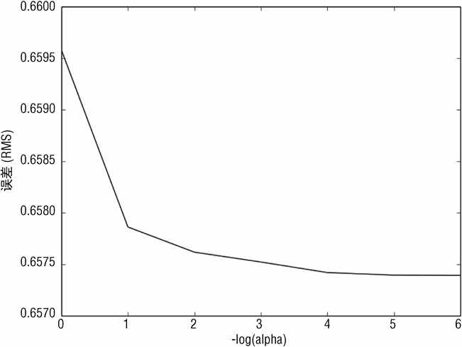
代码清单 3-6 展示了来自岭回归的输出。数字显示岭回归与前向逐步回归有几乎相同的特点。数据更加支持前向逐步回归。
代码清单 3-6 岭回归输出 -ridgeWineOutput.txt
RMS Error alpha
(0.65957881763424564, 1.0)
(0.65786109188085928, 0.1)
(0.65761721446402455, 0.010000000000000002)
(0.65752164826417536, 0.0010000000000000002)
(0.65741906801092931, 0.00010000000000000002)
(0.65739416288512531, 1.0000000000000003e-05)
(0.65739130871558593, 1.0000000000000004e-06)
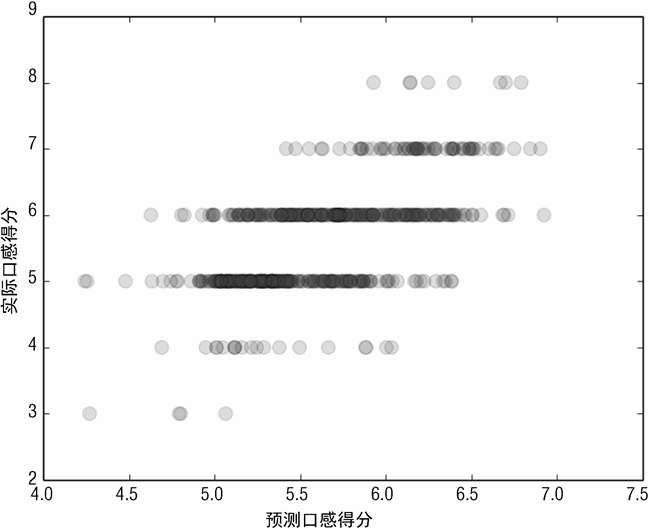
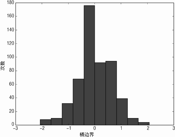
图 3-17 为在红酒数据集上使用岭回归的实际口感得分与预测得分的散点图。图 3-18为预测错误的直方图。
也可以使用更通用的方法来解决分类问题。3.3“度量预测模型性能”讨论了量化分类性能的方法,包括使用误分类错误、不同预测结果的经济代价以及曲线(ROC 曲线)下面积 AUC 来量化性能。
本节使用普通最小二乘法来构建分类器。代码清单 3-7 为相同类型的 Python 代码。与OLS 不同,它使用岭回归作为回归方法(使用一个复杂度控制参数)来构建岩石 - 水雷分类器,使用 AUC 作为分类器的性能度量。代码清单 3-7 类似于红酒品质预测的代码。一个大的区别是代码清单 3-7 使用在测试数据上的预测以及对应的实际结果作为函数 roc_curve(scikit-learn 包中的函数)的输入。这会使得每次训练完成后,AUC 的计算变得更加简单。每个点的错误值经过累加,生成的性能指标被打印出来(参见代码清单 3-8)。
代码清单 3-7 使用岭回归进行岩石 - 水雷分类 -classifierRidgeRocksVMines.py
__author__ = 'mike-bowles'
import urllib2
import numpy
from sklearn import datasets, linear_model
from sklearn.metrics import roc_curve, auc
import pylab as plt
#read data from uci data repository
target_url = ("https://archive.ics.uci.edu/ml/machine-earning-"
"databases/undocumented/connectionist-bench/sonar/sonar.all-data")
data = urllib2.urlopen(target_url)
#arrange data into list for labels and list of lists for attributes
xList = []
labels = []
for line in data:
#split on comma
row = line.strip().split(",")
#assign label 1.0 for "M" and 0.0 for "R"
if(row[-1] == 'M'):
labels.append(1.0)
else:
labels.append(0.0)
#remove lable from row
row.pop()
#convert row to floats
floatRow = [float(num) for num in row]
xList.append(floatRow)
#divide attribute matrix and label vector into training(2/3 of data)
#and test sets (1/3 of data)
indices = range(len(xList))
xListTest = [xList[i] for i in indices if i%3 == 0 ]
xListTrain = [xList[i] for i in indices if i%3 != 0 ]
labelsTest = [labels[i] for i in indices if i%3 == 0]
labelsTrain = [labels[i] for i in indices if i%3 != 0]
#form list of list input into numpy arrays to match input class for
#scikit-learn linear model
xTrain = numpy.array(xListTrain); yTrain = numpy.array(labelsTrain)
xTest = numpy.array(xListTest); yTest = numpy.array(labelsTest)
alphaList = [0.1**i for i in [-3, -2, -1, 0,1, 2, 3, 4, 5]]
aucList = []
for alph in alphaList:
rocksVMinesRidgeModel = linear_model.Ridge(alpha=alph)
rocksVMinesRidgeModel.fit(xTrain, yTrain)
fpr, tpr, thresholds = roc_curve(yTest,rocksVMinesRidgeModel.
predict(xTest))
roc_auc = auc(fpr, tpr)
aucList.append(roc_auc)
print("AUC alpha")
for i in range(len(aucList)):
print(aucList[i], alphaList[i])
#plot auc values versus alpha values
x = [-3, -2, -1, 0,1, 2, 3, 4, 5]
plt.plot(x, aucList)
plt.xlabel('-log(alpha)')
plt.ylabel('AUC')
plt.show()
#visualize the performance of the best classifier
indexBest = aucList.index(max(aucList))
alph = alphaList[indexBest]
rocksVMinesRidgeModel = linear_model.Ridge(alpha=alph)
rocksVMinesRidgeModel.fit(xTrain, yTrain)
#scatter plot of actual vs predicted
plt.scatter(rocksVMinesRidgeModel.predict(xTest),
yTest, s=100, alpha=0.25)
plt.xlabel("Predicted Value")
plt.ylabel("Actual Value")
plt.show()
代码清单 3-8 为 AUC 以及对应的 alpha 值(系数惩罚项的因子)。
代码清单 3-8 使用岭回归得到的岩石 - 水雷分类模型的输出
AUC alpha
(0.84111384111384113, 999.9999999999999)
(0.86404586404586403, 99.99999999999999)
(0.9074529074529073, 10.0)
(0.91809991809991809, 1.0)
(0.88288288288288286, 0.1)
(0.8615888615888615, 0.010000000000000002)
(0.85176085176085159, 0.0010000000000000002)
(0.85094185094185093, 0.00010000000000000002)
(0.84930384930384917, 1.0000000000000003e-05)
AUC 的值接近 1 对应于更好的性能,接近于 0.5 说明效果不太好。使用 AUC 的目标是使其最大化而不是最小化,可以参照之前例子中的 MSE。AUC 在 α =1.0 时有一个明显的突起。数据以及图示显示在 α 远离 1.0 时有明显的下降。回忆一下随着 α 变小,解方案接近于不受限的线性回归问题。α 小于 1.0 时,性能下降表明不受限的解难以达到岭回归的效果。在 3.3 节中,可以看到不受限普通均方回归的结果,其中 AUC 在训练集上的预测性能为 0.98,在测试集上的预测性能为 0.85,非常接近于使用较小的 alpha 的岭回归(α 设为 1E-5)的 AUC 值。这说明岭回归会显著提升性能。
对于岩石 - 水雷问题,数据集包含 60 个属性,总共 208 行数据。将 70 个样本移除作为预留数据,剩下 138 行用于训练。样本数量大约是属性数量的 2 倍,但是不受限解(基于普通的最小二乘法)仍然会过拟合数据。这时使用 10 折交叉验证来估计性能是一个很好的替换方案。使用 10 折交叉验证,每一份数据只有 20 个样本,训练数据相对测试数据就会多很多,从而性能上会有一致的提升。该方法将在第 5 章讨论。
图 3-19 为 AUC 与 alpha 参数的关系,该图展示了在系数向量上使用欧式长度限制可以降低解的复杂度。
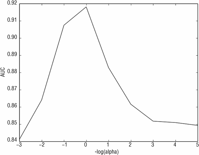
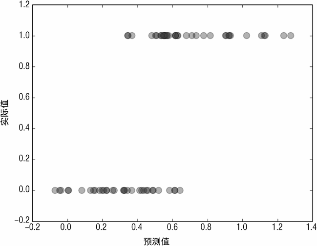
图 3-20 为实际分类结果与分类器预测结果的散点图。该图与红酒预测中的散点图类似。因为实际预测的输出是离散的,所以呈现 2 行水平的点。
本节介绍并探索了普通最小二乘法的 2 种扩展方法、训练以及选择一个现代预测模型的过程。这些扩展方法的介绍有助于理解更普通的惩罚线性回归方法(将在第 4 章中介绍),第 5 章会应用这些方法来解决多个问题。


本书评论